6.2. Working with Matrices

We introduced both vectors and matrices in Vectors and Matrices in MATLAB and discussed how to create them in MATLAB. Here, we present mathematical operations on matrices and review important properties of matrices.

6.2.1. Matrix Math

6.2.1.1. Addition and Subtraction

Addition and subtraction of matrices is performed element-wise.

\[\begin{split}\begin{bmatrix} a & b \\ c & d \end{bmatrix} - \begin{bmatrix} e & f \\ g & h \end{bmatrix} = \begin{bmatrix} a-e & b-f \\ c-g & d-h \end{bmatrix}\end{split}\]

Scalar and element-wise operations between matrices work the same as with vectors. Of course, the size of both matrices must be the same (Element-wise Arithmetic).

6.2.1.2. Matrix Multiplication

Multiplication of a vector by a matrix and multiplication of two matrices are common linear algebra operations. The former is used in the expression of a system of linear equations of the form \(\mathbf{A}\,\bm{x} = \bm{b}\). Points and vectors can be moved, scaled, rotated, or skewed when multiplied by a matrix, which applies to physical geometry and pixels in an image. Later sections explore two primary uses of matrix–to–matrix multiplication. First, we discuss geometric transformation matrices in Geometric Transforms. The transformation matrices are multiplied by the coordinates of points to determine new coordinate locations. Multiplication of the transformation matrices is also used to combine transformations. Secondly, we will cover several matrix factorizations later in this and the following chapters, such as \(\mathbf{A} = \mathbf{L\,U}\), \(\mathbf{A} = \mathbf{Q\,R}\), \(\mathbf{A} = \mathbf{U\,\Sigma\,V}^T\), and \(\mathbf{A} = \mathbf{X\,\Lambda\,X}^{-1}\). Each matrix factorization facilitates solving particular problems. Matrix multiplication verifies that the product of the factors yields the original matrix.

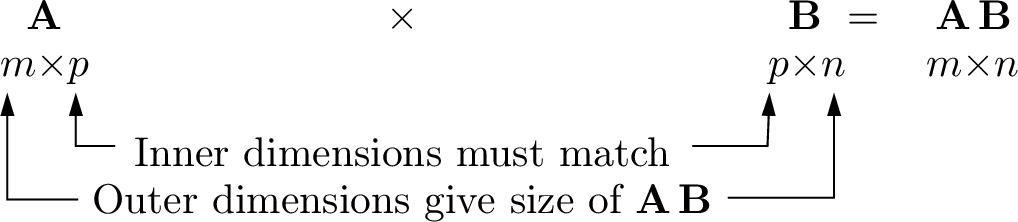
Inner products find the elements of a matrix product. To complete the inner products, the number of columns in the left matrix must match the number of rows in the right matrix. We say that the inner dimensions of the two matrices must agree. As shown in Size of Matrix Multiplications, A \(m{\times}p\) matrix may be multiplied by a \(p{\times}n\) matrix to yield a \(m{\times}n\) matrix. The size of the product matrix is the outer dimensions of the matrices.

Table 6.1 Size of Matrix Multiplications

First Matrix	Second Matrix	Output
\(1{\times}n\) row vector	\(n{\times}1\) column vector	\(1{\times}1\) scalar
\(1{\times}p\) row vector	\(p{\times}n\) matrix	\(1{\times}n\) row vector
\(m{\times}1\) column vector	\(1{\times}n\) row vector	\(m{\times}n\) matrix
\(m{\times}p\) matrix	\(p{\times}1\) column vector	\(m{\times}1\) column vector

Vectors are multiplied by matrices as matrix with only one column (size \(m{\times}1\)). Multiplication of a matrix by a vector is defined as either the linear combination of the columns of the matrix with the vector elements, or as the inner product between the rows of the left matrix and the column vector.

\[\begin{split}\begin{array}{ll} \mathbf{A}\,\bm{x} & = \begin{bmatrix} 1 & 2 & 3 \\ 2 & 5 & 2 \\ 6 & -3 & 1 \end{bmatrix}\, \begin{bmatrix} 2 \\ 1 \\ 1 \end{bmatrix} \\ \\ & = 2\, \begin{bmatrix} 1 \\ 2 \\ 6 \end{bmatrix} + 1\,\begin{bmatrix} 2 \\ 5 \\ -3 \end{bmatrix} + 1\,\begin{bmatrix} 3 \\ 2 \\ 1 \end{bmatrix} \\ \\ & = \begin{bmatrix} 1 & 2 & 3 \\ 2 & 5 & 2 \\ 6 & -3 & 1 \end{bmatrix}\:\begin{bmatrix} 2 \\ 1 \\ 1 \end{bmatrix} \\ \\ & = \begin{bmatrix} 7 \\ 11 \\ 10 \end{bmatrix} \end{array}\end{split}\]

The individual values of a matrix product \(\mathbf{C}_{i,j}\) are calculated as inner products between the rows of the left matrix (\(\bf{A}\)) and the columns of the right matrix (\(\bf{B}\)).

\[\mathbf{C}_{i,j} = \sum_{n=1}^{p} \mathbf{A}_{i,n} \, \mathbf{B}_{n,j}\]

For \(2{\times}2\) matrices:

\[\begin{split}\begin{array}{l} \begin{bmatrix} a & b \\ c & d \end{bmatrix}\, \begin{bmatrix} e & f \\ g & h \end{bmatrix} = \begin{bmatrix} (a\ & e & + & b\ & g) & (a\ & f & + & b\ & h) \\ (c\ & e & + & d\ & g) & (c\ & f & + & d\ & h) \end{bmatrix} \\ \\ \begin{bmatrix} 1 & 2 \\ 3 & 4 \end{bmatrix}\, \begin{bmatrix} 5 & 6 \\ 7 & 8 \end{bmatrix} = \begin{bmatrix} (1\cdot5 & + & 2\cdot7) & (1\cdot6 & + & 2\cdot8) \\ (3\cdot5 & + & 4\cdot7) & (3\cdot6 & + & 4\cdot8) \end{bmatrix} = \begin{bmatrix} 19 & 22 \\ 43 & 50 \end{bmatrix} \end{array}\end{split}\]

6.2.1.3. Matrix Multiplication Properties

1. Matrix multiplication is associative: \((\bf{A\,B})\,\bf{C} = \bf{A}\,(\bf{B\,C})\).

2. In general, matrix multiplication is NOT commutative even for square matrices: (\(\bf{A\,B} \neq \bf{B\,A}\)). Obvious exceptions are multiplication by the identity matrix and an inverse matrix. Note below that the two products of the same matrices are different.

   \[\begin{split}\begin{array}{rl} \begin{bmatrix} 3 & 0 \\ 4 & 3 \end{bmatrix} \begin{bmatrix} 2 & -2 \\ 3 & 4 \end{bmatrix} &= \begin{bmatrix} 6 & -6 \\ 3 & 4 \end{bmatrix} \\ \hfill \\ \begin{bmatrix} 2 & -2 \\ 3 & 4 \end{bmatrix} \begin{bmatrix} 3 & 0 \\ 4 & 3 \end{bmatrix} &= \begin{bmatrix} -2 & -6 \\ 25 & 12 \end{bmatrix} \end{array}\end{split}\]

3. \(\bf{A\,B} = \bf{A\,C}\) does not imply that \(\bf{B} = \bf{C}\). For example, consider matrices:

   \[\begin{split}\begin{array}{c} \mathbf{A} = \begin{bmatrix} 1 & 2 \\ 2 & 4 \end{bmatrix}, \mathbf{B} = \begin{bmatrix} 2 & 1 \\ 1 & 3 \end{bmatrix}, \mathbf{C} = \begin{bmatrix} 4 & 3 \\ 0 & 2 \end{bmatrix} \\ \hfill \\ \mathbf{A\,B} = \mathbf{A\,C} = \begin{bmatrix} 4 & 7 \\ 8 & 14 \end{bmatrix} \end{array}\end{split}\]

6.2.1.4. Matrix Multiplication by Outer Products

We normally think of matrix multiplication as finding each term of the matrix product from the sum of products between the rows of the left matrix and the columns of the right matrix, which is the inner product view of matrix multiplication. But there is also an outer product view that is columns times rows.

\[\begin{split}\mathbf{A\,B} = \begin{bmatrix} \vertbar{} & \vertbar{} & {} & \vertbar{} \\ \bm{a}_1 & \bm{a}_2 & \cdots{} & \bm{a}_p \\ \vertbar{} & \vertbar{} & {} & \vertbar{} \end{bmatrix} \begin{bmatrix} \horzbar{} & \bm{b}_1 & \horzbar{} \\ \horzbar{} & \bm{b}_2 & \horzbar{} \\ {} & \vdots{} & {} \\ \horzbar{} & \bm{b}_p & \horzbar{} \end{bmatrix} = \bm{a}_1\,\bm{b}_1 + \cdots + \bm{a}_p\,\bm{b}_p\end{split}\]

Each \(\bm{a}_k\) column of a \(m{\times}p\) matrix multiplies \(\bm{b}_k\), the \(k\mbox{th}\) row of a \(p{\times}n\) matrix. The product \(\bm{a}_k \bm{b}_k\) is an \(m{\times}n\) rank-one matrix formed from the vector outer product ( Outer Product). The final product \(\bf{A\, B}\) is the sum of the rank-one matrices.

Outer product matrix multiplication gives an alternative perspective of what matrix multiplication accomplishes, which will be useful later when we learn about the singular value decomposition in Singular Value Decomposition (SVD).

6.2.1.5. Matrix Division

In the sense of scalar division, matrix division is not defined for matrices. Multiplication by the inverse of a matrix accomplishes the same objective as division in scalar arithmetic. MATLAB also has two alternative operators to the matrix inverse that act as one might expect from division operators, left-divide (\) and right-divide (/). However, they are more complicated than simple division. As shown in MATLAB’s Matrix Division Operators, they are used to solve systems of linear equations as described in Systems of Linear Equations.

Table 6.2 MATLAB’s Matrix Division Operators

Operator	Name	Need	Usage	Replaces
\	left-divide	A*x = b	x = A\b	x = inv(A)*b
/	right-divide	x*A = b	x = b/A	x = b*inv(A)

6.2.2. Special Matrices

Zero Matrix

A zero vector or matrix contains all zero elements. It is denoted as \(\bf{0}\).

Diagonal Matrix

A diagonal matrix has zeros everywhere except on the main diagonal. Diagonal matrices are usually square (same number of rows and columns), but they may be rectangular with extra rows or columns of zeros.

\[\begin{split}\begin{bmatrix} d_1 & 0 & 0 \\ 0 & d_2 & 0 \\ 0 & 0 & d_3 \end{bmatrix}\end{split}\]

The main diagonal, also called the forward diagonal, or the major diagonal, is the set of diagonal matrix elements from upper left to lower right.

Identity Matrix

An identity matrix (\(\bf{I}\)) is a square, diagonal matrix where all of the diagonal elements are one. Identity matrices are like one in scalar math. The product of any matrix with the identity matrix is itself.

\[\mathbf{A\,I} = \mathbf{A} = \mathbf{I\,A}\]

\[\begin{split}\begin{array}{ll} \mathbf{I}_{2{\times}2} & = \begin{bmatrix} 1 & 0 \\ 0 & 1 \end{bmatrix} \\ \\ \mathbf{I}_{3{\times}3} & = \begin{bmatrix} 1 & 0 & 0 \\ 0 & 1 & 0 \\ 0 & 0 & 1 \end{bmatrix} \\ \\ \mathbf{I}_{4{\times}4} & = \begin{bmatrix} 1 & 0 & 0 & 0 \\ 0 & 1 & 0 & 0 \\ 0 & 0 & 1 & 0 \\ 0 & 0 & 0 & 1 \end{bmatrix} \end{array}\end{split}\]

MATLAB has a function called eye that takes one argument for the matrix size and returns an identity matrix.

>> I2 = eye(2)
I2 =
    1     0
    0     1
>> I3 = eye(3)
I3 =
    1     0     0
    0     1     0
    0     0     1

Upper Triangular Matrix

Upper triangular matrices have all zero values below the main diagonal. Any nonzero elements are on or above the main diagonal.

\[\begin{split}\mathbf{U} = \begin{bmatrix} a & b & c \\ 0 & d & e \\ 0 & 0 & f \end{bmatrix}\end{split}\]

Lower Triangular Matrix

Lower triangular matrices have all zero values above the main diagonal. Any nonzero elements are on or below the main diagonal.

\[\begin{split}\mathbf{L} = \begin{bmatrix} a & 0 & 0 \\ b & c & 0 \\ d & e & f \end{bmatrix}\end{split}\]

Symmetric Matrix

A symmetric matrix (\(\bf{S}\)) has symmetry relative to the main diagonal. If the matrix were written on a piece of paper and you folded the paper along the main diagonal, then the off-diagonal elements with the same value would be at the same position. For symmetric matrices \(\mathbf{S}^T = \mathbf{S}\). Note that for any matrix, \(\bf{A}\), the products \(\mathbf{A}^T\mathbf{A}\) and \(\mathbf{A\,A}^T\) both yield symmetric matrices. Here are two examples of symmetric matrices.

\[\begin{split}\begin{array}{ccc} \begin{bmatrix} 1 & 2 \\ 2 & 3 \end{bmatrix} & \hspace{35pt} & \begin{bmatrix} 2 & 3 & 6 \\ 3 & 1 & 5 \\ 6 & 5 & 2 \end{bmatrix} \end{array}\end{split}\]

Orthonormal Columns

A matrix, \(\bf{Q}\), has orthonormal columns if the columns are unit vectors (length of 1) and the dot product between the columns is zero (\(\cos(\theta) = 0\)). Thus, the columns are orthogonal to each other.

Unitary Matrix

A matrix \(\mathbf{Q} \in \mathbb{C}^{n\,\times\,n}\) is unitary if it has orthonormal columns and is square. The inverse of a unitary matrix is its conjugate (Hermitian) transpose, \(\mathbf{Q}^{-1} = \mathbf{Q}^H\). The product of these matrices with their transpose is the identity matrix, \(\mathbf{Q\,Q}^T = \bf{I}\), and \(\mathbf{Q}^T\,\mathbf{Q} = \bf{I}\).

Orthogonal Matrix

A matrix is orthogonal if its elements are real, \(\mathbf{Q} \in \mathbb{R}^{n\,\times\,n}\), and it is unitary.

Here is an example of multiplication of an orthogonal matrix by its transpose.

\[\begin{split}\begin{array}{lc} & \begin{bmatrix} 0.5 & -0.866 \\ 0.866 & 0.5 \end{bmatrix} \begin{bmatrix} 0.5 & 0.866 \\ -0.866 & 0.5 \end{bmatrix} =\\ \hfill \\ & \begin{bmatrix} {(0.5^2 + 0.866^2)} & {(0.5\cdot0.866 - 0.866\cdot0.5)} \\ {(0.866\cdot0.5 - 0.5\cdot0.866)} & {(0.866^2 + 0.5^2)} \end{bmatrix} = \\ \hfill \\ & \begin{bmatrix} 1 & 0 \\ 0 & 1 \end{bmatrix} \end{array}\end{split}\]

When we discuss the accuracy of solutions to systems of equations (\(\mathbf{A}\,\bm{x} = \bm{b}\)) in Numerical Stability, we will see that the condition number of the \(\bf{A}\) matrix influences the level of obtainable accuracy (Matrix Condition Number). Orthogonal matrices have a condition number of 1, so orthogonal matrix decompositions are used to obtain the most accurate results, especially when \(\bf{A}\) is rectangular (Orthogonal Matrix Decompositions).

6.2.3. Special Matrix Relationships

6.2.3.1. Matrix Inverse

The inverse of a square matrix, \(\bf{A}\), is another matrix, \(\mathbf{A}^{-1}\), that multiplies with the original matrix to yield the identity matrix.

\[\mathbf{A}^{-1} \mathbf{A} = \mathbf{A\,A}^{-1} = \bf{I}\]

Not all square matrices have an inverse, and calculating the inverse for larger matrices is slow.

In MATLAB, the function inv(A) returns the inverse of matrix \(\bf{A}\). MATLAB’s left-divide operator provides a more efficient to using a matrix inverse to solve a system of equations. So while matrix inverses frequently appear in written documentation, we seldom calculate a matrix inverse.

Here are a few properties for matrix inverses.

• \((\mathbf{A\,B})^{-1} = \mathbf{B}^{-1} \mathbf{A}^{-1}\)

  \[\begin{split}\begin{aligned} &(\mathbf{A\,B})^{-1} (\mathbf{A\,B}) = \bf{I} \\ &(\mathbf{A\,B})^{-1} \mathbf{A\,B\,B}^{-1} \mathbf{A}^{-1} = \bf{I} \mathbf{B}^{-1} \mathbf{A}^{-1} \\ &(\mathbf{A\,B})^{-1} = \mathbf{B}^{-1} \mathbf{A}^{-1} \end{aligned}\end{split}\]

• \({\left( \mathbf{A}^T \right) }^{-1} = {\left( \mathbf{A}^{-1} \right) }^{T}\).

  Start with the simple observation that \(\mathbf{I}^T = \bf{I}\) and \((\mathbf{A\,B})^T = \mathbf{B}^T \mathbf{A}^T\) ( Matrix Transpose Properties).

  \[\begin{split}\begin{array}{rl} &{\left( \mathbf{A}^{-1} \mathbf{A} \right)}^T = \mathbf{I}^T = \mathbf{I} \\ &\mathbf{A}^T {\left( \mathbf{A}^{-1} \right)}^T = \mathbf{I} \\ &{\left( \mathbf{A}^T \right)}^{-1} \mathbf{A}^T {\left( \mathbf{A}^{-1} \right)}^T = {\left( \mathbf{A}^T \right)}^{-1} \\ &{\left( \mathbf{A}^{-1} \right)}^T = {\left( \mathbf{A}^T \right)}^{-1} \end{array}\end{split}\]

6.2.3.2. Matrix Transpose Properties

We described the transpose for vectors and matrices in Transpose.

• \({\left( \mathbf{A}^{T} \right)}^T = \bf{A}\)

• The transpose with respect to addition, \((\mathbf{A} + \mathbf{B})^T = \mathbf{A}^T + \mathbf{B}^T\).

• \((\mathbf{A\,B})^T = \mathbf{B}^T \, \mathbf{A}^T\). Notice that the order is reversed.

  \[\begin{split}\begin{array}{rcl} (i, j) \mbox{ value of } (\mathbf{A\,B})^T & = & (j, i) \mbox{ value of } \mathbf{A\,B} \\ & = & j \mbox{ row of } \mathbf{A} \times i \mbox{ column of } \mathbf{B} \\ & = & i \mbox{ row of } \mathbf{B}^T \times j \mbox{ column of } \mathbf{A}^T \\ & = & (i, j) \mbox{ value of } \mathbf{B}^T\,\mathbf{A}^T \end{array}\end{split}\]

• We often pre-multiply vectors and matrices by their transpose (\(\mathbf{A}^T \mathbf{A}\)). The result is a scalar for a column vector, and a square, symmetric matrix for a row vector, rectangular matrix, and square matrix. If \(\mathbf{A}\) is a \(m{\times}n\) matrix, \(\mathbf{A}^T \mathbf{A}\) is a \(n{\times}n\) square, symmetric matrix.

  Since \(\mathbf{S} = \mathbf{A}^T \mathbf{A}\) is symmetric, then \(\mathbf{S}^T = \mathbf{S}\).

  \[\mathbf{S}^T = {\left( \mathbf{A}^T \mathbf{A} \right)}^T = \mathbf{A}^T {\left( \mathbf{A}^T \right)}^T = \mathbf{A}^T \mathbf{A} = \mathbf{S}\]

  Another interesting result is that the trace of \(\mathbf{S} = \mathbf{A}^T \mathbf{A}\), denoted as \(Tr(\mathbf{S})\), is the sum of the squares of all the elements of \(\bf{A}\). The trace of a matrix is the sum of its diagonal elements.

  \[\begin{split}\mathbf{A}^T\mathbf{A} = \begin{bmatrix} a & b & c \\ d & e & f \end{bmatrix} \begin{bmatrix} a & d \\ b & e \\ c & f \end{bmatrix} = \begin{bmatrix} {a^2 + b^2 + c^2} & {ad + be + cf} \\ {ad + be + cf} & {d^2 + e^2 + f^2} \end{bmatrix}\end{split}\]

• For unitary matrices, \(\mathbf{Q}^H = \mathbf{Q}^{-1}\).

  Spectral Theorem

  Theorem 6.1 (Spectral Theorem)

  When a matrix is unitary with orthonormal columns, the matrix’s Hermitian transpose is the matrix’s inverse, \(\mathbf{Q}^H = \mathbf{Q}^{-1}\).

  Proof. Since the columns are unit vectors, it follows that the diagonal of \(\mathbf{Q}^T \mathbf{Q}\) is ones. The off-diagonal values are zeros because the dot product between the columns is zero. Thus,

  \[\begin{split}\begin{array}{l} \mathbf{Q}^T \mathbf{Q} = \mathbf{Q\,Q}^T = \mathbf{I} \\ \hfill \\ \mathbf{Q}^T = \mathbf{Q}^{-1} \end{array}\end{split}\]

  For complex unitary matrices, the complex conjugates of the Hermitian transpose ensure that the \(\m{Q\,Q}^H = \m{Q}^H \m{Q} = \m{I}\) is real.

  \(\qed\)

  Here is an example of an orthogonal rotation matrix.

  >> Q
  Q =
      0.5000   -0.8660
      0.8660    0.5000
  
  >> Q'
  ans =
      0.5000    0.8660
     -0.8660    0.5000
  
  % column dot product
  >> Q(:,1)'*Q(:,2)
  ans =
      0
  % orthogonal columns
  >> Q'*Q
  ans =
      1.0000   -0.0000
     -0.0000    1.0000
  
  % orthogonal rows
  >> Q*Q'
  ans =
      1.0000    0.0000
      0.0000    1.0000
  

  Another interesting result about orthogonal matrices is that the product of two orthogonal matrices is also orthogonal because both the inverse and transpose of matrices reverse the matrix order. Proof of orthogonality only requires that \(\mathbf{Q}^T = \mathbf{Q}^{-1}\).

  Consider two orthogonal matrices \(\mathbf{Q}_1\) and \(\mathbf{Q}_2\).

  \[{\left(\mathbf{Q}_1 \mathbf{Q}_2 \right)}^{-1} = \mathbf{Q}_2^{-1} \mathbf{Q}_1^{-1} = \mathbf{Q}_2^T \mathbf{Q}_1^T = {\left(\mathbf{Q}_1 \mathbf{Q}_2 \right)}^T\]

• When a transpose is made of a matrix with complex values, we usually also take the complex conjugate of each value, which is called a Hermitian transpose. The conjugate of each value is often needed in numerical algorithms because when a complex number is multiplied by its conjugate, the product is a real number. The complex matrix product \(\mathbf{S} = \mathbf{A}^H\,\mathbf{A}\) is said to be Hermitian. Hermitian matrices have real numbers along the diagonal, and the other values are symmetric conjugates. In technical writing, the Hermitian transpose is usually indicated as \(\mathbf{A}^H\). In some older publications, it may be written as \(\mathbf{A}^*\) or even as \(\mathbf{A}^{\dagger}\). Also in technical writing, symmetric matrices that may or may not have complex values are usually referred to as Hermitian rather than symmetric.

  In MATLAB, A’ is the Hermitian transpose of A. While A.’ is the transpose of A, where the complex conjugates of the values in A are not taken. The two transposes achieve the same result when the matrix is real.

6.2.4. Determinant

The determinant of a square matrix is a number. At one time, determinants were a significant component of linear algebra. But that is not so much the case today [STRANG99]. Determinants are now more important for analytical than computational purposes. Thus, while knowing the application of determinants is important, we will avoid using them when possible.

• Either of two notations is used to indicate the determinant of a matrix, \(\det(\bf{A})\) or \(\vert\bf{A}\vert\).

• The classic technique for computing a determinant is called the Laplace expansion. The complexity of computing a determinant by the classic Laplace expansion method has run-time complexity on the order of \(n!\) (n–factorial), which is slow for large matrices.

• In practice, the determinant for matrices is computed using a faster method that is described in Determinant Shortcut and improves the performance to \(\mathcal{O}(n^3)\). [1] The faster method uses the result that \(\det(\mathbf{A\,B)} = \det(\mathbf{A})\,\det(\mathbf{B})\). The LU decomposition factors are computed as described in LU Decomposition, then the determinant is the product of the determinants of the LU decomposition factors.

The determinant of a \(2{\times}2\) matrix is simple, but it gets more complicated as the matrix size increases.

\[\begin{split}\begin{vmatrix} a & b \\ c & d \end{vmatrix} = a\,d - c\,b\end{split}\]

The \(n{\times}n\) determinant requires \(n\) determinants, called cofactors, each of size \((n-1){\times}(n-1)\). In each stage of Laplace expansion, the elements in a row or column are multiplied by a cofactor determinant from the other rows and columns, excluding the row and column of the multiplication element. The determinant is then the sum of the expansion along the chosen row or column. But then the \((n-1){\times}(n-1)\) determinants need to be calculated. It works as follows for a \(3{\times}3\) determinant.

\[\begin{split}\begin{vmatrix} a & b & c \\ d & e & f \\ g & h & i \end{vmatrix} = a\, \begin{vmatrix} e & f \\ h & i \end{vmatrix} - b\, \begin{vmatrix} d & f \\ g & i \end{vmatrix} + c\, \begin{vmatrix} d & e \\ g & h \end{vmatrix}\end{split}\]

Another approach to remembering the sum of products needed to compute a \(3{\times}3\) determinant is to append the first two columns and then compute diagonal product terms. The left-to-right terms are added, while the right-to-left terms are subtracted. Note: This only works for \(3{\times}3\) determinants.

\[\begin{split}\begin{array}{rl} \begin{vmatrix} a & b & c \\ d & e & f \\ g & h & i \end{vmatrix} &= \begin{vmatrix} a & {} & b & {} & c & {} & a & {} & b \\ {} & \diagdown & {} & \diagdown & {} & \diagdown & {} & {} & {} \\ d & {} & e & {} & f & {} & d & {} & e \\ {} & {} & {} & \diagdown & {} & \diagdown & {} & \diagdown & {} \\ g & {} & h & {} & i & {} & g & {} & h \end{vmatrix} \\ & \hfill \\ &- \begin{vmatrix} a & {} & b & {} & c & {} & a & {} & b \\ {} & {} & {} & \diagup & {} & \diagup & {} & \diagup & {} \\ d & {} & e & {} & f & {} & d & {} & e \\ {} & \diagup & {} & \diagup & {} & \diagup & {} & {} & {} \\ g & {} & h & {} & i & {} & g & {} & h \end{vmatrix} \end{array}\end{split}\]

\[\begin{split}\begin{vmatrix} a & b & c \\ d & e & f \\ g & h & i \end{vmatrix} = aei + bfg + cdh - ceg - afh - bdi\end{split}\]

For a \(4{\times}4\) determinant, the pattern continues with each cofactor term now being a \(3{\times}3\) determinant. The pattern likewise continues for higher-order matrices. The number of computations needed with this method of computing a determinant is on the order of \(n!\), which is prohibitive for large matrices.

Notice that the sign of the cofactor additions alternates according to the pattern:

\[\begin{split}sign_{i,j} = (-1)^{i+j} = \begin{bmatrix} + & - & + & - \\ - & + & - & + \\ + & - & + & - \\ - & + & - & + \end{bmatrix}\end{split}\]

It is not necessary to always use the top row for Laplace expansion. Any row or column will work, but note the cofactors’ signs. The best strategy is to apply Laplace expansion along the row or column with the most zeros.

Here is a bigger determinant problem with many zeros, so it is not too bad. At each expansion stage, there is a row or column with only one nonzero element, so finding the sum of cofactor determinants is unnecessary.

\[\begin{split} \begin{array}{rl} \begin{vmatrix} 8 & 5 & 4 & 3 & 0 \\ 7 & 0 & 6 & 1 & 0 \\ 8 & -5 & 4 & 3 & -5 \\ -3 & 0 & 0 & 0 & 0 \\ 4 & 0 & 2 & 2 & 0 \end{vmatrix} &= 3 \times \begin{vmatrix} 5 & 4 & 3 & 0 \\ 0 & 6 & 1 & 0 \\ -5 & 4 & 3 & -5 \\ 0 & 2 & 2 & 0 \end{vmatrix} \\ \hfill \\ = 3 \times 5 \times \begin{vmatrix} 5 & 4 & 3 \\ 0 & 6 & 1 \\ 0 & 2 & 2 \end{vmatrix} &= 3 \times 5 \times 5 \times \begin{vmatrix} 6 & 1 \\ 2 & 2 \end{vmatrix} = 750 \end{array}\end{split}\]

MATLAB has a function called det that takes a square matrix as input and returns the determinant.

6.2.5. Calculating a Matrix Inverse

The inverse of a square matrix, \(\bf{A}\), is another matrix, \(\mathbf{A}^{-1}\) that multiplies with the original matrix to yield the identity matrix.

\[\mathbf{A}^{-1} \mathbf{A} = \mathbf{A}\,\mathbf{A}^{-1} = \bf{I}\]

Unfortunately, calculating the inverse of a matrix is computationally slow. A formula known as Cramer’s Rule provides a succinct equation for the inverse, but it is prohibitively slow for matrices beyond a \(2{\times}2\). Cramer’s rule requires the calculation of the determinant and the full set of cofactors for the matrix. Cofactors are determinants of matrices one dimension less than the original matrix. To find the inverse of a \(3{\times}3\) matrix requires finding one \(3{\times}3\) determinant and 9 \(2{\times}2\) determinants. The run time complexity of Cramer’s rule is \(\mathcal{O}(n\cdot\,n!)\).

For a \(2{\times}2\) matrix, Cramer’s rule can be found by algebraic substitution.

\[\begin{split}\begin{array}{rl} \mathbf{A\,A}^{-1} &= \bf{I} \\ \begin{bmatrix} a & b \\ c & d \end{bmatrix} \begin{bmatrix} x_1 & x_2 \\ y_1 & y_2 \end{bmatrix} &= \begin{bmatrix} 1 & 0 \\ 0 & 1 \end{bmatrix} \end{array}\end{split}\]

One can perform the above matrix multiplication and find four simple equations from which the terms of the matrix inverse may be derived.

\[\begin{split}\mathbf{A} = \begin{bmatrix} a & b \\ c & d \end{bmatrix} \mbox{ has inverse } \mathbf{A}^{-1} = \frac{ \begin{bmatrix} d & -b \\ -c & a \end{bmatrix}} {det(\mathbf{A})} = \frac{1}{(a\,d - c\,b)} \begin{bmatrix} d & -b \\ -c & a \end{bmatrix}\end{split}\]

Because of the computational complexity, Cramer’s rule is not used by MATLAB or similar software. The good news is that we do not need to manually calculate the inverse of matrices because MATLAB has a matrix inverse function called inv. MATLAB’s inv function finds the inverse by first finding the singular value decomposition ( Singular Value Decomposition (SVD)). The factors of the SVD are orthogonal and diagonal, so their inverse is quick to determine.

>> A = [2 -3 0;4 -5 1;2 -1 -3];
>> A_inv = inv(A)
A_inv =
    -1.6000    0.9000    0.3000
    -1.4000    0.6000    0.2000
    -0.6000    0.4000   -0.2000

Note

For square matrices, the left-divide operator uses an efficient elimination technique called LU decomposition to solve a system of equations. Thus, it is seldom necessary to compute the full inverse of the matrix.

6.2.6. Invertible Test

Not all matrices can be inverted. A matrix that is said to be singular is not invertible. A matrix is singular if some of its rows or columns are dependent on each other. An invertible matrix must derive from the same number of independent equations as the number of unknown variables. A square matrix from independent equations has rank equal to the dimension of the matrix, and is said to be full rank. The rank of a matrix is the number of independent rows and columns in the matrix.

Vector Spaces gives more formal definitions of independent and dependent vectors and describes how the rank of a matrix is calculated.

The following matrix is singular because column 3 is just column 1 multiplied by 2.

\[\begin{split}\begin{bmatrix} 1 & 0 & 2 \\ 2 & 1 & 4 \\ 1 & 2 & 2 \end{bmatrix}\end{split}\]

When a matrix is singular, its rank is less than the dimension of the matrix, and its determinant also evaluates to zero.

>> A = [1 0 2;2 1 4;1 2 2];
>> rank(A)
ans =
     2
>> det(A)
ans =
    0
>> det(A')  % the transpose is also singular
ans =
    0

Using MATLAB, you will occasionally see a warning message that a matrix is close to singular. The message may also reference a rcondition number. The condition and rcondition numbers indicate if a matrix is invertible, which we will describe in Matrix Condition Number. We will focus on the rank as our invertible test for our discussion here.

6.2.7. Cross Product

The cross product is a special operation using two vectors in \(\mathbb{R}^3\) with application to geometry and physical systems.

The cross product of two nonparallel 3-D vectors is a vector perpendicular to both vectors and the plane they span, and is called the normal vector to the plane. The direction of the normal vector follows the right-hand rule as shown in figure Fig. 6.11. Finding the normal vector to a plane is needed to write the equation of a plane. Projections Onto a Hyperplane shows an example of using a cross product to find the equation of a plane.

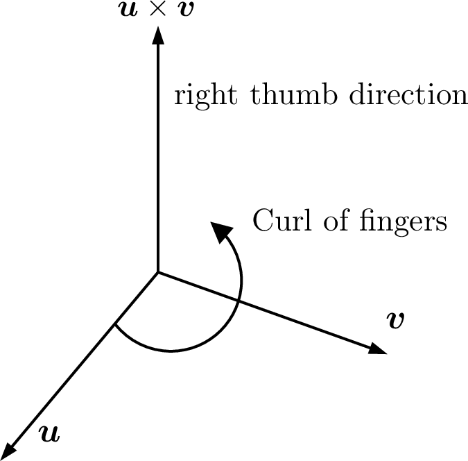
Fig. 6.11 Right Hand Rule: \(\bm{u} \times \bm{v}\) points in the direction of your right thumb when the fingers curl from \(\bm{u}\) to \(\bm{v}\).

• \(\bm{u} \times \bm{v}\) is spoken as “\(\bm{u}\) cross \(\bm{v}\)”.

• \(\bm{u} \times \bm{v}\) is perpendicular to both \(\bm{u}\) and \(\bm{v}\).

• \(\bm{v} \times \bm{u}\) is \(-(\bm{u} \times \bm{v})\).

• The length \(\norm{\bm{v} \times \bm{u}} = \norm{\bm{u}}\,\norm{\bm{v}}\,|\sin \theta|\), where \(\theta\) is the angle between \(\bm{u}\) and \(\bm{v}\).

• The MATLAB function cross(u, v) returns \(\bm{u} \times \bm{v}\).

Cross Product by Determinant

The cross product of \(\bm{u} = (u_1, u_2, u_3)\) and \(\bm{v} = (v_1, v_2, v_3)\) is a vector.

\[\begin{split}\begin{array}{ll} \bm{u} \times \bf{v} & = \begin{vmatrix} \vec{i} & \vec{j} & \vec{k} \\ u_1 & u_2 & u_3 \\ v_1 & v_2 & v_3 \end{vmatrix} \\ \\ & = \vec{i}(u_2 v_3 - u_3 v_2) - \vec{j}(u_1 v_3 - u_3 v_1) + \vec{k}(u_1 v_2 - u_2 v_1) \end{array}\end{split}\]

Vectors \(\vec{i}\), \(\vec{j}\), and \(\vec{k}\) are the unit vectors in the directions of \(\bm{x}\), \(\bm{y}\), and \(\bm{z}\) of the 3-D axis.

Cross Product by Skew-Symmetric Multiplication

An alternative way to compute \(\bm{u} \times \bm{v}\) is by multiplication of a skew-symmetric, or anti-symmetric matrix.

• The skew-symmetric matrix of \(\bm{u}\) is given the math symbol, \([\bm{u}]_\times\). Such a matrix has a zero diagonal and is always singular. The transpose of a skew-symmetric matrix is equal to its negative.

  \[[\bm{u}]_{\times}^T = -[\bm{u}]_{\times}\]

• MATLAB function skew(u) returns \([\bm{u}]_\times\).

• For vectors in \(\mathbb{R}^3\):

  \[\begin{split}[\bm{u}]_\times = \begin{bmatrix} 0 & -u_3 & u_2 \\ u_3 & 0 & -u_1 \\ -u_2 & u_1 & 0 \end{bmatrix}\end{split}\]
  \[\bm{u} \times \bm{v} = [\bm{u}]{_\times}\,\bm{v}\]

>> u = [1 2 3]';
>> v = [1 0 1]';
>> cross(u,v)
ans =
    2
    2
   -2
>> s = skew(u)
s =
    0    -3     2
    3     0    -1
   -2     1     0
>> s*v
ans =
    2
    2
   -2

[1]

The symbol \(\mathcal{O}(\,)\) is called Big–O. It is a measure of the order of magnitude of the number of calculations needed relative to the size of the data operated on, \(n\). If we say that an algorithm has a run-time complexity of \(\mathcal{O}(n^3)\), we are not saying that \(n^3\) is the exact number of calculations needed to run the algorithm. Rather, we are saying that the order of magnitude of the number of calculations needed has a cubic relationship to \(n\). So if the number of data elements is doubled, then the number of calculations needed grows by a factor of 8, \(\mathcal{O}((2n)^3)\).