6.4. Systems of Linear Equations

Systems of linear equations are everywhere in the systems that engineers design. Many (probably most) systems are linear. Differential equations sometimes describe systems, but we can change differential equations to linear equations by applying the Laplace transform. The main point, though, is that in actual design and analysis applications, we have systems of equations with multiple unknown variables, not just one equation. We will consider some application examples of systems of linear equations in Linear System Applications. Initially, we will focus on how to solve them.

The variables in linear equations are only multiplied by numbers. We do not have products of variables such as \(xy\) or \(x^2\). We also do not have exponentials such as \(e^x\) or functions of variables.

6.4.1. An Example

The following system of equations has three unknown variables.

\[\begin{split}\left\{\begin{aligned} 2\,x_1 - 3\,x_2 {\quad \quad} &= 3 \\ 4\,x_1 - 5\,x_2 + x_3 &= 9 \\ 2\,x_1 - x_2 - 3\,x_3 &= -1 \end{aligned}\right.\end{split}\]

The first step is to represent the equations as a matrix equation.

\[\begin{split} \begin{bmatrix} 2 & -3 & 0 \\ 4 & -5 & 1 \\ 2 & -1 & -3 \end{bmatrix} \begin{bmatrix} x_1 \\ x_2 \\ x_3 \end{bmatrix} = \begin{bmatrix} 3 \\ 9 \\ -1 \end{bmatrix}\end{split}\]

The common notation for describing this equation is \(\mathbf{A}\,\bm{x} = \bm{b}\), where the vector \(\bm{x}\) represents the unknowns. In linear algebra notation, we describe the solution to the problem in terms of the inverse of the \(\bf{A}\) matrix, which is discussed in Calculating a Matrix Inverse, and

Elimination to Find the Matrix Inverse. Note that we have to be careful about the order of the terms because matrix multiplication is not commutative.

(6.10)\[\begin{split} \mathbf{A}^{-1}\,\mathbf{A}\,\bm{x} = \bm{x} = \mathbf{A}^{-1}\,\bm{b} \\\end{split}\]

We can find the solution this way with the inv function, but MATLAB provides a more efficient way to solve it.

6.4.2. Jumping Ahead to MATLAB

The left-divide operator (\) solves systems of linear equations more efficiently than multiplying by the inverse of a matrix.

>> A = [2 -3 0; 4 -5 1; 2 -1 -3];
>> b = [3 9 -1]';
>> x = A\b
x =
    3.0000
    1.0000
    2.0000

Thus, the values of the three unknown variables are: \(x_1 = 3\), \(x_2 = 1\), and \(x_3 = 2\).

MATLAB’s left-divide operator is a complete solution to any linear system of equations. We will take a quick look at how the left-divide operator (also known as the mldivide function) evaluates the form of the \(\bf{A}\) matrix to determine which algorithms to use to solve the matrix equation. Even though MATLAB gave us a powerful and versatile function for solving systems of linear equations, we still want to understand the algorithms it uses and in what situations each is appropriate. Engineers need to understand MATLAB’s results to make correct conclusions, and for cases where MATLAB or similar software is not available. In learning how to solve linear systems, we will also gain knowledge about data analysis and other applications of linear algebra beyond systems of equations.

Challenge: Your Own Linear System Solver

Developing an independent implementation of an algorithm is a good way to understand how an algorithm works. To help you learn more as you read this chapter, you might write your linear system solver similar to MATLAB’s left-divide operator. Start with diagonal and triangular solvers. Later, after reading the corresponding sections, add LU decomposition and Cholesky decomposition for square matrices. Use the SVD to estimate the condition number of the matrix. Finally, add the QR decomposition algorithms to solve rectangular systems.

6.4.3. When Does a Solution Exist?

Not every matrix equation of the form \(\mathbf{A}\,\bm{x} = \bm{b}\) has a unique solution. A few tests can help determine if a unique solution exists. The matrix in question here has \(m\) rows and \(n\) columns (\(m{\times}n\)).

Solutions to systems of equations of the form \(\mathbf{A}\,\bm{x} = \bm{b}\), may:

1. Be an exact, unique solution, which occurs with both critically-determined (square) and over-determined systems of equations.

2. Not exist, which can occur with any system of equations, but is usually associated with square, singular systems of equations.

3. Not exist, but can be approximated, which occurs with over-determined systems of equations.

4. Be an infinite set of vectors, which occurs with under-determined systems of equations.

A square matrix system has a unique solution when the following five conditions hold for the matrix \(\bf{A}\). If one of the conditions holds, they all hold. If any condition is false, then all conditions are false and the matrix \(\bf{A}\) is singular and no solution to \(\mathbf{A}\,\bm{x} = \bm{b}\) exists [WATKINS10].

1. \(\mathbf{A}^{-1}\) exists.

2. There is no nonzero \(\bm{x}\) such that \(\mathbf{A}\,\bm{x} = \bm{0}\).

3. The \(\bf{A}\) matrix is full rank, \(\text{rank}(\mathbf{A}) = m = n\). The columns and rows of \(\bf{A}\) are linearly independent.

4. \(\det(\mathbf{A}) \neq 0\). The determinant is a well-known test for \(\bf{A}\) being invertible (not singular), but it is slow for larger matrices. The previous rank test is sufficient.

5. For any given vector \(\bm{b}\), there is exactly one vector \(\bm{x}\) such that \(\mathbf{A}\,\bm{x} = \bm{b}\).

The next example does not have a solution because the third row of \(\bf{A}\) is a linear combination of rows 1 and 2 (4*A(2,:) + A(1,:)).

>> A = [1 2 3; 0 3 1; 1 14 7];
>> % A is not full rank
>> rank(A)
ans =
    2
>> % Not invertible
>> det(A)
ans =
    0
>> b = [1; 2; 3];
>> % This won't go well
>> A \ b
Warning: Matrix is singular
to working precision.
ans =
    NaN
   -Inf
    Inf

The next example has a better result.

\[\begin{split} \begin{bmatrix} 5 & 6 & -1 \\ 6 & 3 & 2 \\ -2 & -3 & 6 \end{bmatrix}\,\begin{bmatrix} x_1 \\ x_2 \\ x_3 \end{bmatrix} = \begin{bmatrix} 8 \\ 0 \\ 8 \end{bmatrix}\end{split}\]

>> A = [5 6 -1;
        6 3 2; -2 -3 6];
>> b = [8 0 8]';
>> rank(A)   % full rank
ans =
    3
>> x = A \ b
x =
   -2.8889
    4.1481
    2.4444

6.4.4. Column and Row Factorization

A matrix factoring converts a matrix into two or more sub-matrices whose product yields the original matrix. Matrix factorization, or decomposition, is quite common in linear algebra and is used when the submatrices are needed for implementing algorithms. Here, we present a factorization that is not used in any algorithms. Its purpose is solely to provide information and, more importantly, to facilitate learning about systems of equations. It is not part of MATLAB, but the code is listed below. The CR (for column–row) factoring of matrix \(\bf{A}\) produces matrix \(\bf{C}\) that consists of the independent columns of \(\bf{A}\) and another matrix, \(\bf{R}\), showing how combinations of the columns of \(\bf{C}\) are used in \(\bf{A}\) [MOLER20]. The CR factoring was proposed by Dr. Gilbert Strang [1] of the Massachusetts Institute of Technology [STRANG20]. The CR factorization aims to illustrate concepts related to independent and dependent columns and how dependent columns degrade systems of equations.

function [C,R] = cr(A)
% [C,R] = cr(A) is Strang's column-row factorization, A = C*R.
% If A is m-by-n with rank r, then C is m-by-r and R is r-by-n.

    [R,j] = rref(A);
    r = length(j);     % r = rank.
    R = R(1:r,:);
    C = A(:,j);
end

The cr function uses the rref function to perform Gaussian elimination as described in Reduced Row Echelon Form. For now, consider the output of cr rather than its implementation.

The matrix in the following example has independent columns. So in the CR factoring, the \(\bf{C}\) matrix is the same as \(\bf{A}\). The \(\bf{R}\) matrix is an identity matrix, indicating that each column of \(\bf{C}\) is found unchanged in \(\bf{A}\). Matrices with independent rows and columns are said to be full rank.

>> A = randi(10, 3);
A =
    3    10     8
    6     2     7
   10    10    15
>> [C, R] = cr(A)
C =
    3    10    10
    6     2     5
   10    10     9
R =
    1     0     0
    0     1     0
    0     0     1

Rank

The rank, \(r\), of a matrix is the number of independent rows and columns of the matrix. Rank is never more than the smaller dimension of the matrix.

The CR factoring helps us to see if some rows or columns are linear combinations of other rows or columns. The cr function shows one way to compute a matrix’s rank: the number of nonzero pivot variables from the elimination algorithm, which are the diagonal elements of \(\bf{R}\). See Vector Spaces and

Rank from the SVD for more information on calculating a matrix’s rank.

Now we change the \(\bf{A}\) matrix, making the third column a linear combination of the first two. The rank of the matrix is then 2. We can see the rank from the CR factorization as the number of columns in \(\bf{C}\) and the number of rows in \(\bf{R}\). The last column of \(\bf{R}\) shows how the first two columns of \(\bf{C}\) combine to make the third column of \(\bf{A}\).

>> A(:,3) = A(:,1) + A(:,2)/2
A =
    3    10     8
    6     2     7
   10    10    15
>> [C, R] = cr(A)
C =
    3    10
    6     2
   10    10
R =
    1.0000         0    1.0000
         0    1.0000    0.5000

6.4.5. The Row and Column View

A system of linear equations may be viewed from either the perspective of its rows or columns. Plots of row line equations and column vectors give us a geometric understanding of systems of linear equations. The row view shows each row as a line, with the solution being the point where the lines intersect. The column view shows each column as a vector and presents the solution as a linear combination of the column vectors. The column view yields a perspective that will be particularly useful when we consider over-determined systems.

Let’s illustrate the two views with a simple example.

\[\begin{split}\left\{\begin{matrix} 2x & + & y & = & 4 \\ -x & + & y & = & 1 \end{matrix}\right.\end{split}\]

\[\begin{split}\begin{bmatrix} 2 & 1 \\ -1 & 1 \end{bmatrix} \begin{bmatrix} x \\ y \end{bmatrix} = \begin{bmatrix} 4 \\ 1 \end{bmatrix}\end{split}\]

To find the solution, we can either use the left-divide operator or elimination, which is discussed in Elimination.

\[\begin{split}\begin{bmatrix} 2 & 1 \\ -1 & 1 \end{bmatrix} \begin{bmatrix} 1 \\ 2 \end{bmatrix} = \begin{bmatrix} 4 \\ 1 \end{bmatrix}\end{split}\]

Row View Plot

We rearrange our equations into line equations.

\[\begin{split}\left\{\begin{matrix} y & = & -2x & + & 4 \\ y & = & x & + & 1 \end{matrix}\right.\end{split}\]

As shown in figure Fig. 6.18, the point where the lines intersect is the solution to the system of equations. Two parallel lines represent a singular system that does not have a solution.

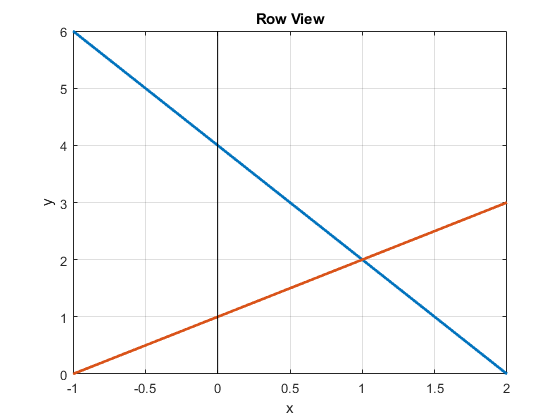
Fig. 6.18 In the row view of a system of equations, the solution is where the line equations intersect.

If another row (equation) is added to the system, making it over-determined, an exact solution can still be found if the new row is consistent with the existing rows. For example, we could add the equation \(3x + 2y = 7\) to the system, and the line plot for the new equation will intersect the other lines at the same point, so \(x = 1; y = 2\) is still valid. We could still say that \(\bm{b}\) is in the column space of \(\bf{A}\). Of course, most rows that might be added will not be consistent with the existing rows, so we can only approximate a solution, which we will cover in Over-determined Systems and Vector Projections.

Column View Plot

Let’s view the system of equations as a linear combination of column vectors.

\[\begin{split}1 \times \begin{bmatrix} 2 \\ -1 \end{bmatrix} + 2 \times \begin{bmatrix} 1 \\ 1 \end{bmatrix} = \begin{bmatrix} 4 \\ 1 \end{bmatrix}\end{split}\]

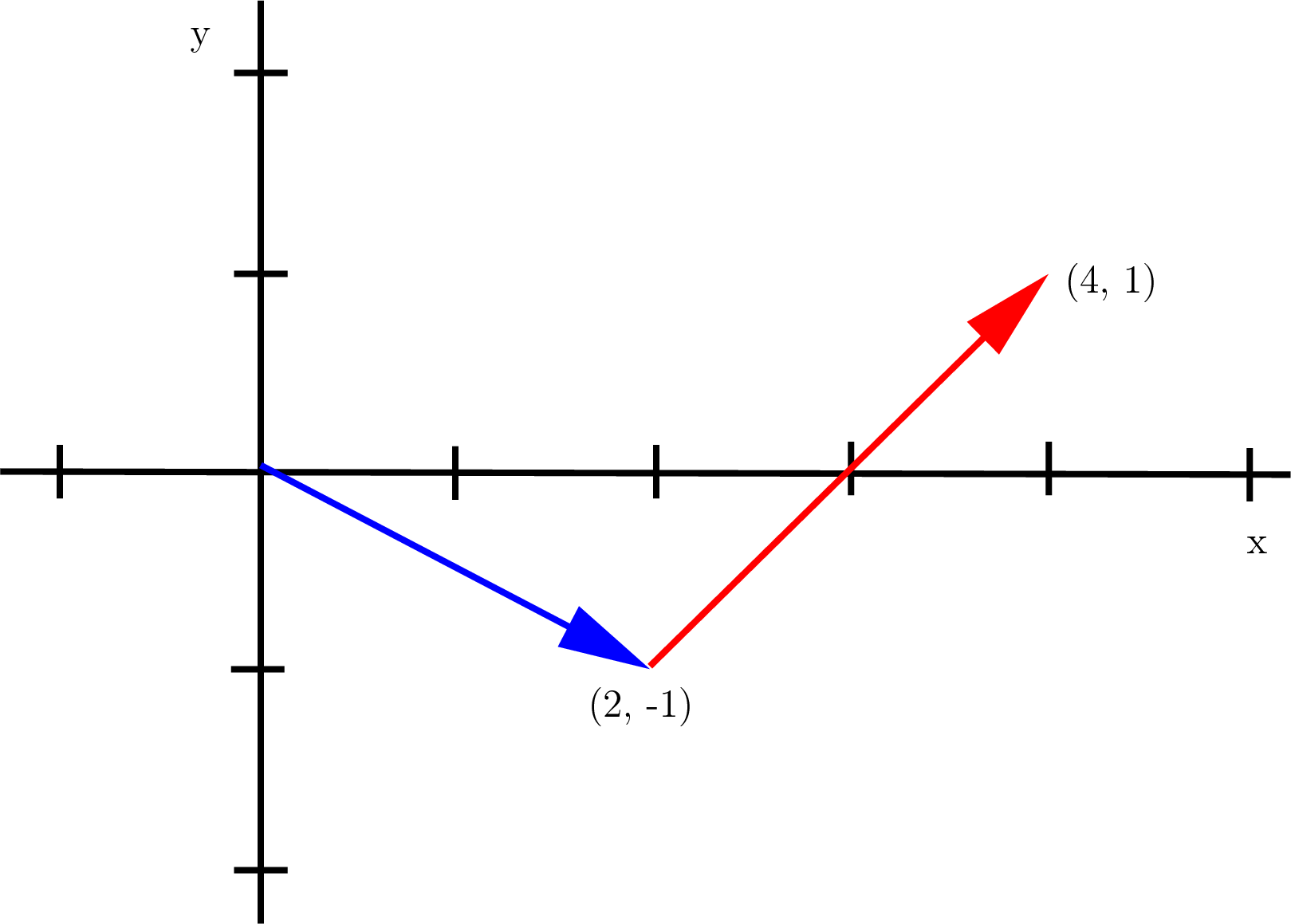
Fig. 6.19 The column view shows a linear combination of the column vectors. Each vector is scaled such that the sum of the vectors is the same as the vector on the right side of the equation.

As depicted in figure Fig. 6.19, there is a nonzero linear combination of the column vectors of a full rank matrix that can reach any point in the vector space except the origin. When \(\bf{A}\) is full rank and vector \(\bm{b}\) is nonzero, then \(\bm{b}\) is always in the column space of \(\bf{A}\). The all-zero multipliers provide the only way back to the origin for a full rank system. But a singular system with parallel vectors can have a nonzero vector leading back to the origin, which is called the null solution (Null Space).

In the Column Space of \(\bf{A}\)

Consider the columns of a matrix \(\bf{A}\) as vectors. The set of vectors that can be formed from linear combinations of the vectors is called the span of the columns of \(\bf{A}\). A vector that is part of the span of the columns is said to be in the column space of \(\bf{A}\), a phrase with particular relevance to over-determined systems.

Note

Now complete Matrix Homework.

Footnote

[1]

Dr. Gilbert Strang is widely considered to be a leading authority and advocate for teaching applications of linear algebra science and engineering.