6.1. Working with Vectors

Vectors and Matrices in MATLAB defines how to create and use vectors in MATLAB. Here, we define some linear algebra operations on vectors.

Vectors have scalar coefficients defining their displacement in each dimension of a coordinate axis system. We can think of a vector as having a specific length and direction. What we don’t always know about a vector is where it begins. Lacking other information about a vector, we can consider that the vector begins at the origin. Points are sometimes confused with vectors because they are also defined by a set of coefficients for each dimension. The values of points are always relative to the origin. Vectors may be defined as spanning between two points (\(\bm{v} = \mathbf{p}_1 - \mathbf{p}_2\)).

Figure Fig. 6.1 shows the relationship of points and vectors relative to the coordinate axes.

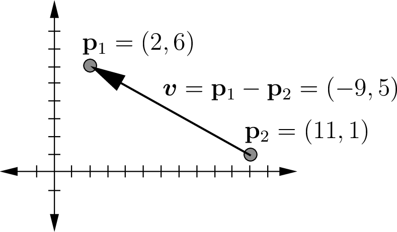
Fig. 6.1 The elements of points are the coordinates relative to the axes. The elements of vectors tell the length of the vector for each dimension.

Note that vectors are usually stored as column vectors in MATLAB. One might accurately observe that the data of a vector is a set of numbers, which is neither a row vector nor a column vector [KLEIN13]. However, MATLAB stores vectors as either row vectors or column vectors. The need to multiply a vector by a matrix using inner products (defined in Dot Product or Inner Product) motivates using column vectors. Because column vectors take more space when displayed in written material, they are often displayed in one of two alternate ways—either as the transpose of a row vector \([a, b, c]^T\) or with parentheses \((a, b, c)\).

Note

The word vector comes from the Latin word meaning “carrier”.

6.1.1. Linear Vectors

Vectors are linear, which, as shown in figure Fig. 6.2, means that they can be added together (\(\bm{u} + \bm{v}\)) and scaled by multiplication by a scalar constant (\(k\,\bm{v}\)). Vectors may also be defined as a linear combination of other vectors (\(\bm{x} = 3\,\bm{u} + 5\,\bm{v}\)).

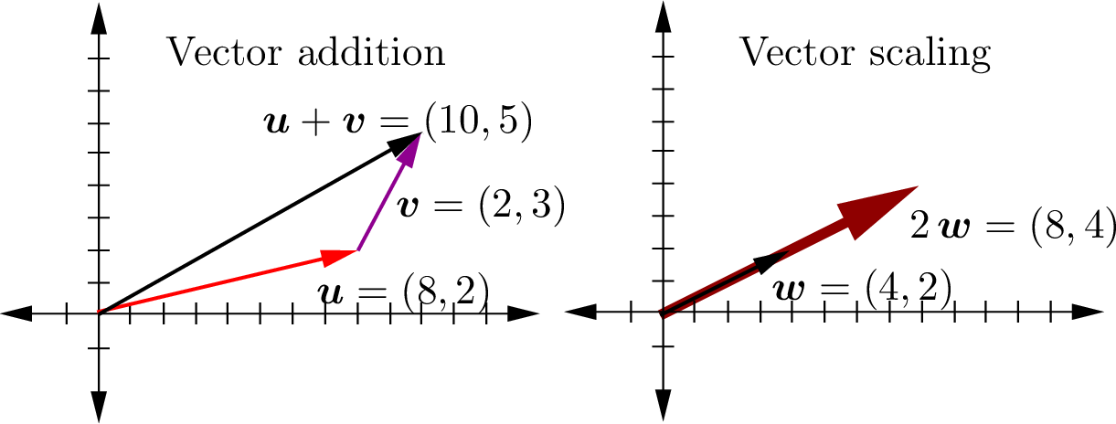
Fig. 6.2 Examples of vector addition and vector scaling

6.1.2. Independent Vectors

A vector is independent of other vectors within a set if no linear combination of other vectors defines the vector. Consider the following set of four vectors.

\[\begin{split}\left\{ \underbrace{\begin{bmatrix} 1 \\ 2 \\ 2 \end{bmatrix}}_{\bm{w}}, \; \underbrace{\begin{bmatrix} 3 \\ -6 \\ 4 \end{bmatrix}}_{\bm{x}}, \; \underbrace{\begin{bmatrix} 5 \\ -2 \\ 8 \end{bmatrix}}_{\bm{y}}, \; \underbrace{\begin{bmatrix} 9 \\ -2 \\ 1 \end{bmatrix}}_{\bm{z}} \right\}\end{split}\]

The first three vectors of the set \(\{\bm{w},\,\bm{x},\, \mbox{and}\, \bm{y}\}\) are not independent because \(\bm{y} = 2\,\bm{w} + \bm{x}\). Likewise, \(\bm{w} = \frac{1}{2}(\bm{y} - \bm{x})\) and \(\bm{x} = \bm{y} - 2\,\bm{w}\). However, \(\bm{z}\) is independent of the other three vectors.

Sometimes we can observe dependent relationships, but it is often difficult to see them. MATLAB has a few functions that will help one test for independence and even see the dependent relationships. Tests for independence include the rank and det functions discussed in

Invertible Test. The rref (Reduced Row Echelon Form) and cr functions (Column and Row Factorization) show the relationships between dependent vectors. The cr function is not part of MATLAB, but is described in Column and Row Factorization. Vector Spaces gives a more mathematically formal definition of linearly independent vectors.

6.1.3. Transpose

The transpose of either a vector or a matrix reverses the rows and columns.

\[\begin{split}\begin{array}{l} \mbox{Let } \bm{a} = \begin{bmatrix} a \\ b \\ c \end{bmatrix} \mbox{ then, } \bm{a}^T = \begin{bmatrix} a & b & c \end{bmatrix} \\ \hfill \\ \mbox{Let } \bm{b} = \begin{bmatrix} a & b & c \end{bmatrix} \mbox{ then, } \bm{b}^T = \begin{bmatrix} a \\ b \\ c \end{bmatrix} \\ \hfill \\ \mbox{Let } \mathbf{C} = \begin{bmatrix} a & b & c \\ d & e & f \end{bmatrix} \mbox{then, } \mathbf{C}^T = \begin{bmatrix} a & d \\ b & e \\ c & f \end{bmatrix} \end{array}\end{split}\]

In MATLAB, the transpose operator is the apostrophe (’):

>> A_trans = A';

Note

The .’ operator performs a simple transpose, and ’ performs a complex conjugate transpose, also referred to as a Hermitian transpose. The result of the two operators is the same for matrices with only real numbers. For matrices with complex numbers, the complex conjugate is usually desired. In mathematical literature, the simple transpose is almost always represented as \(({\cdot})^T\), and the Hermitian transpose may be denoted as \({(\cdot})^H\), \({(\cdot)}^*\), or \({(\cdot)}^{(\dagger)}\).

6.1.4. Dot Product or Inner Product

The sum of products between the elements of two vectors is called a dot product. The operation yields a scalar.

\[\begin{split} &\begin{bmatrix} a \\ b \\ c \end{bmatrix} \cdot \begin{bmatrix} d \\ e \\ f \end{bmatrix} = a\,d + b\,e + c\,f \\ \hfill \\ &\begin{bmatrix} 1 \\ 2 \\ 3 \end{bmatrix} \cdot \begin{bmatrix} 4 \\ 5 \\ 6 \end{bmatrix} = 1\cdot4 + 2\cdot5 + 3\cdot6 = 32\end{split}\]

Inner Product

An inner product is the sum of products between a row vector and a column vector. The multiply operator (*) in MATLAB performs an inner product. Thus, to calculate a dot product, we only need to multiply the transpose of the first vector by the second vector. The resulting scalar is the dot product of the vectors.

For example,

\[\begin{split}\begin{array}{l} \begin{array}{lr} \bm{a} = \begin{bmatrix} 1 \\ 2 \end{bmatrix} & \bm{b} = \begin{bmatrix} 3 \\ 4 \end{bmatrix} \end{array} \\ \begin{array}{ll} \bm{a} \cdot \bm{b} & = \bm{a}^T\,\bm{b} = \begin{bmatrix} 1 & 2 \end{bmatrix} \begin{bmatrix} 3 \\ 4 \end{bmatrix} \\ & = 1\cdot3 + 2\cdot4 \\ & = 11 \end{array} \end{array}\end{split}\]

The inner product is also used to calculate the product of matrices. Each element of the product is an inner product between a row of the left matrix and a column of the right matrix.

MATLAB has a dot function that takes two vector arguments and returns the scalar dot product. However, implementing a dot product using inner product multiplication is often just as easy.

>> a = [3; 5];
>> b = [2; 4];
>> c = dot(a,b)
c =
    26

>> c = a'*b
c =
    26

Note

If the vectors are both row vectors (nonstandard), then the dot product becomes \(\bm{a} \cdot \bm{b} = \bm{a} \, \bm{b}^T\).

6.1.5. Dot Product Properties

6.1.5.1. Commutative

The dot product \(\bm{u} \cdot \bm{v}\) equals \(\bm{v} \cdot \bm{u}\). The order does not matter.

6.1.5.2. Length of Vectors

The length of the vector \(\bm{v}\), \(\norm{\bm{v}}\), is the square root of the dot product of \(\bm{v}\) with itself.

\[\norm{\bm{v}} = \sqrt{\bm{v} \cdot \bm{v}} = (v_1^2 + v_2^2 + ... + v_n^2)^{1/2}\]

MATLAB has a function called norm that takes a vector as an argument and returns the length. The Euclidean length of a vector is called the \(l_2\)-norm, which is the default for the norm function. See Norms for information on other vector length measurements.

A normalized or unit vector is a vector of length one. A vector may be normalized by dividing it by its length.

\[\bm{\hat{v}} = \frac{\bm{v}}{\norm{\bm{v}}}\]

6.1.5.3. Angle Between Vectors

Consider two unit vectors (length 1) in \(\mathbb{R}^2\) as shown in figure Fig. 6.3, \(\bm{u} = (1, 0)\) and \(\bm{v} = (\cos \theta, \sin \theta)\). Then consider the same vectors rotated by an angle \(\alpha\), such that \(\theta = \beta - \alpha\).

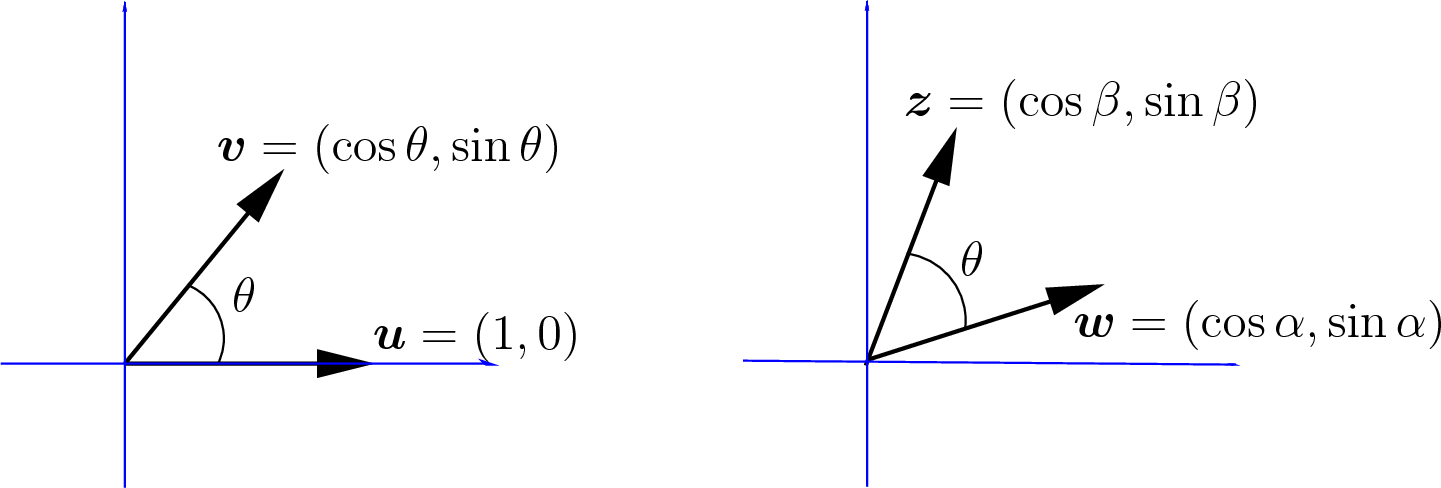
Fig. 6.3 The dot product between two unit vectors is the cosine of the angle between the vectors.

(6.1)\[\begin{split}\begin{array}{ll} \bm{u} \cdot \bm{v} & = 1 \cdot \cos \theta + 0 \cdot \sin \theta = \cos \theta \\ \bm{w} \cdot \bm{z} & = \cos \alpha \cdot \cos \beta + \sin \alpha \cdot \sin \beta \\ & = \cos(\beta - \alpha) \\ & = \cos \theta \end{array}\end{split}\]

The result of equation (6.1) can also be found from the law of cosines, which tells us that

\[\norm{\bm{z} - \bm{w}}^2 = \norm{\bm{z}}^2 + \norm{\bm{w}}^2 - 2\norm{\bm{z}}\,\norm{\bm{w}} \cos \theta\]

Since both \(\bm{z}\) and \(\bf{w}\) are unit vectors, several terms become 1.

\[\begin{split}\begin{array}{rl} (\bm{z} - \bm{w}) \cdot (\bm{z} - \bm{w}) &= 2 - 2\,\cos \theta \\ \bm{z}\cdot\bm{z} - 2\,\bm{w}\cdot\bm{z} + \bm{w}\cdot\bm{w} &= 2 - 2\,\cos \theta \\ - 2\,\bm{w}\cdot\bm{z} &= - 2\,\cos \theta \\ \bm{w}\cdot\bm{z} &= \cos \theta \end{array}\end{split}\]

When the vectors are not unit vectors, the vector lengths are constants.

\[\left( \frac{\bm{v}}{\norm{\bm{v}}} \right) \cdot \left( \frac{\bm{w}}{\norm{\bm{w}}} \right) = \cos \theta\]

(6.2)\[\boxed{\bm{v} \cdot \bm{w} = \norm{\bm{v}} \, \norm{\bm{w}} \cos \theta}\]

All angles have \(\abs{\cos \theta} \leq 1\). So all vectors have:

\[\abs{\bm{v} \cdot \bm{w}} \leq \norm{\bm{v}}\,\norm{\bm{w}}\]

6.1.5.4. Orthogonal Vector Test

When two vectors are perpendicular (\(\theta = \pi/2\) or 90°), then from equation (6.2) their dot product is zero. The property extends to \(\mathbb{R}^3\) and beyond, where we say that the vectors in \(\mathbb{R}^n\) are orthogonal when their dot product is zero.

The geometric properties of orthogonal vectors provide useful strategies for finding optimal solutions for some problems. One example of this is demonstrated in Over-determined Systems and Vector Projections.

Perpendicular Vectors

By the Pythagorean theorem, if \(\bm{u}\) and \(\bm{v}\) are perpendicular, then as shown in figure Fig. 6.4, \(\norm{\bm{u}}^2 + \norm{\bm{v}}^2 = \norm{\bm{u} - \bm{v}}^2\).

>> u = [0; 1];
>> v = [1; 0];
>> w = v - u
w =
    1
   -1
>> v'*v + u'*u
ans =
    2
>> w'*w
ans =
    2

Fig. 6.4 Dot products and the Pythagorean theorem

6.1.6. Applications of Dot Products

6.1.6.1. Perpendicular Rhombus Vectors

As illustrated in figure Fig. 6.5, a rhombus is any parallelogram whose sides are the same length. Let us use the properties of dot products to show that the diagonals of a rhombus are perpendicular.

Fig. 6.5 A rhombus is a parallelogram whose sides are the same length. The dot product can show that the diagonals of a rhombus are perpendicular.

Matrix Transpose Properties lists transpose properties, including the transpose of a vector sum, \((\bm{a} + \bm{b})^T = \bm{a}^T + \bm{b}^T\). We also need to use the fact that the sides of a rhombus are the same length. We begin by setting the dot product of the diagonals equal to zero.

(6.3)\[\begin{split}\begin{array}{rl} (\bm{u} + \bm{v})^T\,(\bm{u} - \bm{v}) &= 0 \\ (\bm{u}^T + \bm{v}^T)\,(\bm{u} - \bm{v}) &= 0 \\ \bm{u}^T\bm{u} - \bm{u}^T\bm{v} + \bm{v}^T\bm{u} - \bm{v}^T\bm{v} &= 0 \\ \bm{u}^T\bm{u} &= \bm{v}^T\bm{v} \\ \end{array}\end{split}\]

Each term of equation (6.3) is a scalar, and dot products are commutative, so the middle two terms cancel each other, and we are left with the requirement that the lengths of the sides of the rhombus be the same, which is in the definition of a rhombus.

6.1.6.2. Square Corners

When building something in the shape of a rectangle, we want the four corners to be square (perpendicular). A common test to verify that the corners are square is to measure the length of the diagonals between opposite corners. If the corners are square, then the lengths of the diagonals will be equal. Here we will prove that the test is valid.

With reference to figure Fig. 6.6, we want to show that \(\norm{\bm{u} + \bm{v}} = \norm{\bm{u} - \bm{v}}\). The dot product of a vector with itself gives the length squared, which, if equivalent, proves that the lengths are equivalent. Recall that \(\bm{u}^T\bm{v}\) and \(\bm{v}^T\bm{u}\) are equal scalar values.

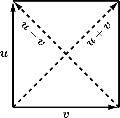
Fig. 6.6 A rectangle with four square corners

(6.4)\[\begin{split}\begin{array}{rl} (\bm{u} + \bm{v})^T\,(\bm{u} + \bm{v}) &= (\bm{u} - \bm{v})^T\,(\bm{u} - \bm{v}) \\ (\bm{u}^T + \bm{v}^T)\,(\bm{u} + \bm{v}) &= (\bm{u}^T - \bm{v}^T)\,(\bm{u} - \bm{v}) \\ \bm{u}^T\bm{u} + \bm{u}^T\bm{v} + \bm{v}^T\bm{u} + \bm{v}^T\bm{v} &= \bm{u}^T\bm{u} - \bm{u}^T\bm{v} - \bm{v}^T\bm{u} + \bm{v}^T\bm{v} \\ 2\,\bm{u}^T\bm{v} &= -2\,\bm{u}^T\bm{v} \end{array}\end{split}\]

Several terms of equation (6.4) cancel out. Equation (6.4) can only be true when \(\bm{u}^T\bm{v} = -\bm{u}^T\bm{v} = 0\), which is only satisfied when \(\bm{u}\) and \(\bm{v}\) are perpendicular (\(\bm{u} \perp \bm{v}\)).

6.1.6.3. Find a Perpendicular Vector

Let us consider a mobile robotics problem. The robot needs to execute a wall-following algorithm. We will use two of the robot’s distance sensors. One is perpendicular to the robot’s direction of travel, and one is at 45°. As shown in figure Fig. 6.7, we establish points \(\bf{p}_1\) and \(\bf{p}_2\) from the sensors in the robot’s coordinate frame along the wall and find vector \(\bm{b} = \bf{p}_2 - \bf{p}_1\). We need to find a short-term goal location for the robot to drive toward that is perpendicular to the wall at a distance of \(k\) from the point \(\bf{p}_2\). Using vectors \(\bm{a}\) and \(\bm{b}\), we can find an equation for vector \(\bm{c}\) such that \(\bm{c}\) is perpendicular to \(\bm{b}\), and \(\bm{c}\) begins at the origin of \(\bm{a}\). With the coordinates of \(\bm{c}\), the goal location is a simple calculation.

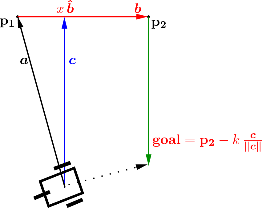
Fig. 6.7 Finding vector \(\bm{c}\) perpendicular to the wall, \(\bm{b}\), is needed to find the wall–following goal location.

We want to identify the vector from the terminal point of \(\bm{a}\) to the terminal point of \(\bm{c}\) as \(\bm{\hat{b}}\,x\) where \(x\) is a scalar and \(\bm{\hat{b}}\) is a unit vector in the direction of \(\bm{b}\).

\[\bm{\hat{b}} = \frac{\bm{b}}{\norm{\bm{b}}}\]

(6.5)\[\bm{c} = \bm{a} + \bm{\hat{b}}\,x\]

We find the answer by starting with the orthogonality requirement between vectors \(\bm{c}\) and \(\bm{\hat{b}}\).

\[\begin{split}\begin{array}{rl} \bm{\hat{b}}^T (\bm{a} + \bm{\hat{b}}\,x) &= 0 \\ \bm{\hat{b}}^T\bm{a} + \bm{\hat{b}}^T\bm{\hat{b}}\,x &= 0 \\ x &= - \bm{\hat{b}}^T\bm{a} \end{array}\end{split}\]

Since \(\bm{\hat{b}}\) is a unit vector, \(\bm{\hat{b}}^T\bm{\hat{b}} = 1\) and drops out of the equation. We return to equation (6.5) to find the equation for \(\bm{c}\).

(6.6)\[\bm{c} = \bm{a} - \bm{\hat{b}\,\hat{b}}^T \bm{a}\]

Figure Fig. 6.8 shows an example starting with the sensor measurements for points \(\mathbf{p}_1\) and \(\mathbf{p}_2\). Finding the vector \(\bm{c}\) perpendicular to the wall with equation (6.6) makes finding the short-term goal location quite simple. We are using sensors on the robot at \(\pm 90^{\circ}\) and \(\pm 45^{\circ}\), and the coordinate frame is that of the robot’s, so \(\mathbf{p}_1\) is on the \(y\) axis and \(\mathbf{p}_2\) is on a line at \(\pm 45^{\circ}\) from the robot. The robot begins 50 cm from the wall.

>> p1 = [0; 50];
>> p2 = [40; 40];
>> b = p2 - p1;
>> bhat = b/norm(b);
>> a = p1;
>> c = a - bhat*(bhat'*a);
>> k = 50;
>> goal = p2 - k*c/norm(c)
goal =
    27.873
    -8.507

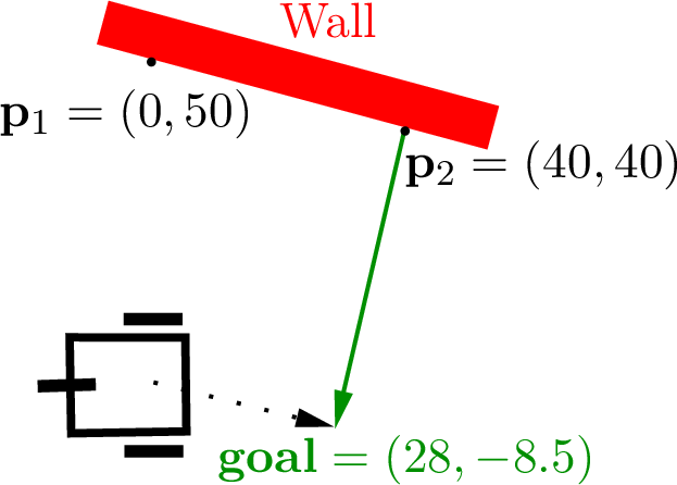
Fig. 6.8 Wall–following example

6.1.7. Outer Product

Whereas the inner product (dot product) of two vectors is a scalar (\(\bm{u} \cdot \bm{v} = \bm{u}^T\,\bm{v}\)), the outer product of two vectors is a matrix. Each element of the outer product is a product of an element from the left column vector and an element from the right row vector. Outer products are not used nearly as often as inner products, but in Singular Value Decomposition (SVD) we will see an important application of outer products.

\[\begin{split}\bm{u} \otimes \bm{v} = \bm{u\,v}^T = \begin{bmatrix} u_1 \\ u_2 \\ \vdots \\ u_m \end{bmatrix} \begin{bmatrix} v_1 & v_2 & \cdots & v_n \end{bmatrix} = \begin{bmatrix} u_1v_1 & u_1v_2 & \cdots & u_1v_n \\ u_2v_1 & u_2v_2 & \cdots & u_2v_n \\ \vdots & \vdots & \ddots & \vdots \\ u_mv_1 & u_mv_2 & \cdots & u_mv_n \end{bmatrix}\end{split}\]

6.1.8. Dimension and Space

Basis vectors provide the coordinate axes used to define the coordinates of points and vectors. The \(\mathbb{R}^2\) Cartesian basis vectors are defined by the two columns of the identity matrix, \((1, 0)\) and \((0, 1)\). A plot of a portion of the Cartesian \(\mathbb{R}^2\) vector space is shown in figure Fig. 6.9.

>> c_basis = eye(2)
c_basis =
     1     0
     0     1

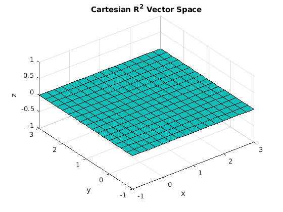
Fig. 6.9 The 2-dimensional Cartesian vector space is a plane where \(z = 0, \forall (x, y)\).

A vector space consists of a set of vectors and a set of scalars that are closed under vector addition and scalar multiplication. Saying that they are closed means that we can add any vectors in the vector space together and multiply any vectors in the space by a scalar, and the resulting vectors are still in the vector space. The set of all possible vectors in a vector space is called the span of the vector space.

For example, vectors in our physical 3-dimensional world are said to be in a vector space called \(\mathbb{R}^3\). Vectors in \(\mathbb{R}^3\) consist of three real numbers defining their magnitude in the \(\bm{x}\), \(\bm{y}\), and \(\bm{z}\) directions. Similarly, vectors on a 2-D plane, like a piece of paper, are said to be in the vector space called \(\mathbb{R}^2\).

Let us clarify a subtle matter of definitions. We normally think of the term dimension as how many coordinate values are used to define points and vectors, which is accurate for coordinates relative to their basis vectors. However, when points in a custom coordinate system are mapped to Cartesian coordinates via multiplication by the basis vectors, then the number of elements matches the number of elements in the basis vectors rather than the number of basis vectors. In Vector Spaces, we define dimension more precisely as the number of basis vectors in the vector space.

In figure Fig. 6.10, a \(\mathbb{R}^2\) custom vector space has basis vectors as the columns of the \(\bf{W}\) matrix. Even though the basis vectors are in \(\mathbb{R}^3\) Cartesian coordinates, the vector space is 2-dimensional since there are two basis vectors, and the span of the vector space is a plane.

Notice that the two basis vectors are orthogonal to each other. Since the basis vectors are in the columns of \(\bf{W}\), the equation \(\mathbf{W}^T\,\mathbf{W} = \mathbf{I}\) verifies that the columns are orthogonal.

>> W
W =
    0.8944   -0.0976
         0    0.9759
    0.4472    0.1952
>> point = [1; 2];
>> cartesian = W*point
cartesian =
    0.6992
    1.9518
    0.8376
>> W'*W
ans =
    1.0000    0.0000
    0.0000    1.0000

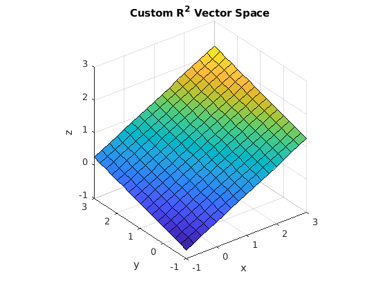
Fig. 6.10 Two custom basis vectors define a 2-dimensional vector space.

Other vector spaces may also be used for applications unrelated to geometry and may have higher dimensions than 3. Generally, we call this \(\mathbb{R}^n\). For some applications, the coefficients of the vectors and scalars may also be complex numbers, which is a vector space denoted as \(\mathbb{C}^n\).