6.11.2. Projections Onto a Hyperplane
We can extend projections to \(\mathbb{R}^3\) and still visualize the projection as projecting a vector onto a plane. Here, the column space of matrix \(\bf{A}\) is two 3-dimension vectors, \(\bm{a}_1\) and \(\bm{a}_2\).
The span of two vectors in \(\mathbb{R}^3\) forms a plane. As before, we have an approximation solution to \(\mathbf{A}\,\bm{x} = \bm{b}\), which can be written as \(\mathbf{A}\,\bm{\hat{x}} = \bm{p}\). The error is \(\bm{e} = \bm{b} - \bm{p} = \bm{b} - \mathbf{A}\,\bm{\hat{x}}\). We want to find \(\bm{\hat{x}}\) such that \(\bm{b} - \mathbf{A}\,\bm{\hat{x}}\) is orthogonal to the plane, so again we set the dot products equal to zero.
The left matrix is just \(\mathbf{A}^T\), which is size \(2{\times}3\). The size of \(\bm{\hat{x}}\) is \(2{\times}1\), so the size of \(\mathbf{A}\,\bm{\hat{x}}\), like \(\bm{b}\), is \(3{\times}1\).
As with the vector projection solution of equation (6.27), equation (6.28) minimizes the error for over-determined systems of equations. The orthogonal solution makes use of QR decomposition. When \(\bf{A}\) in equation (6.28) is replaced with \(\mathbf{Q\, R}\), two matrix products reduce to the identity matrix.
Because \(\bf{A}\) is over-determined, the last \(m - n\) rows of \(\bf{R}\) will be all zeros, so we can reduce the size of \(\bf{Q}\) and \(\bf{R}\) with the economy QR option where only the first \(n\) columns of \(\bf{Q}\) are returned. \(\bf{Q}\) is now \(m{\times}n\), and \(\bf{R}\) is \(n{\times}n\). After finding \(\bf{Q}\) and \(\bf{R}\), computing the solution only requires one \(n{\times}m\) multiplication with a \(m{\times}1\) vector and then a \(n{\times}n\) back-substitution of an upper triangular matrix.
In MATLAB, we can find \(\hat{\bm{x}}\) as:
x_hat = (A'*A) \ (A'*b);

% or

[Q, R] = qr(A, 0); % Economy QR
x_hat = R \ (Q'*b);
Note
(A \ b) finds the same answer. The left-divide operator handles
under-determined, over-determined, and square matrix systems
Left-Divide Operator).
The projection vector is then:
The projection matrix is:
Note
\(\bf{A}\) is not a square matrix and thus is not invertible. If it were, \(\mathbf{P} = \bf{I}\) and there would be no need to do the projection. Try to verify why this is the case. Recall that \((\mathbf{BA})^{-1} = \mathbf{A}^{-1}\mathbf{B}^{-1}\).
6.11.2.1. Over-determined Pseudo-inverse
Recall from our discussion of square matrices that while we might write the solution to \(\mathbf{A}\,\bm{x} = \bm{b}\) as \(\bm{x} = \mathbf{A}^{-1} \bm{b}\), that is not how we should compute \(\bm{x}\) because computing the matrix inverse is slow. However, a one-time calculation based only on \(\bf{A}\) should be considered when we need to compute multiple solutions with a fixed \(\bf{A}\) matrix and different \(\bm{b}\)’s. We have two ways to achieve this objective that are preferred over computing the inverse of \(\bf{A}\) by elimination. One option is an LU decomposition of \(\bf{A}\) and reuse of \(\bf{L}\) and \(\bf{U}\) with a triangular solver for each \(\bm{b}\). We could also compute the inverse of \(\bf{A}\) from the SVD as shown in Singular Value Decomposition.
Similarly, we sometimes need a one-time calculation on rectangular systems that we can reuse. This is the Moore–Penrose pseudo-inverse of \(\bf{A}\), which we denote as \(\bf{A}^+\), and \(\bm{x} = \mathbf{A}^+ \bm{b}\) is the least squares (minimum length) solution to \(\mathbf{A}\,\bm{x} = \bm{b}\).
We have already found from projections that equation (6.31) is the least squares solution, but it has unacceptable computational performance.
Computing \(\mathbf{A}^{T}\mathbf{A}\) is slow if \(\bf{A}\) is large and the multiplication degrades the condition of the system. Although a solution using the Cholesky solver is reasonable if \(\bf{A}\) is not too large, strategies based on orthogonal matrix factorizations are preferred.
Several matrix multiplications simplify to the identity matrix if we let \(\mathbf{A} = \mathbf{Q\, R}\) or \(\mathbf{A} = \mathbf{U\,\Sigma\, V}^T\) in equation (6.31).
The solutions using the QR and SVD factors in equation (6.32) are
equivalent since computing the pseudo-inverse of \(\bf{R}\) results
in an SVD calculation. By Orthogonally Equivalent Matrices in
Golub–Kahan 1965, matrices \(\bf{A}\) and \(\bf{R}\) are
orthogonally equivalent. So if
\(\mathbf{R}^+ = \mathbf{V\,\Sigma}^+\,\mathbf{U}_r^T\), then
\(\mathbf{A}^+ = \mathbf{V\,\Sigma}^+\,\left(\mathbf{U}_r^T \mathbf{Q}^T\right)\)
is an equivalent equation to \(\mathbf{A}^+\) from the SVD of
\(\bf{A}\) in equation (6.32). MATLAB uses the SVD to
calculate the pseudo-inverses of both over-determined system and
under-determined systems (The Preferred Under-determined Solution). The MATLAB function is
called as Aplus = pinv(A).
Since \(\bf{\Sigma}\) is a diagonal matrix, its inverse is the reciprocal of the nonzero elements on the diagonal. Refer to equation (8.4) in Properties of Eigenvalues and Eigenvectors. The zero elements remain zero.
>> S = diag([2 3 0])
S =
    2     0     0
    0     3     0
    0     0     0
>> pinv(S)
ans =
    0.5000         0         0
         0    0.3333         0
         0         0         0
Here is an example of using the pseudo-inverse on an over-determined matrix equation. Note that the full SVD calculation is not needed here. The economy SVD (Economy SVD) is sufficient.
>> A=randi(20,15,4)-8;
>> y=randi(10,4,1)-4
y =
     4
    -1
     2
     3
>> b = A*y;
>> [U, S, V] = svd(A, 'econ');
>> pinvA=V*pinv(S)*U';
>> x = pinvA*b
x =
    4.0000
   -1.0000
    2.0000
    3.0000
>> x = pinv(A)*b
x =
    4.0000
   -1.0000
    2.0000
    3.0000
6.11.2.2. Projection Example
The projectR3 script and the resulting plot in figure
Fig. 6.27 demonstrate the calculation and display
of a vector’s projection onto the matrix’s column space. The dot product
is also calculated to verify orthogonality.
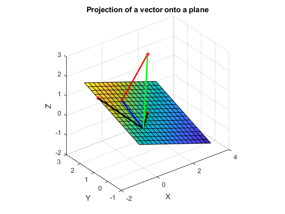
Fig. 6.27 The projection of a vector onto the column space of \(\bf{A}\), which spans a plane in \(\mathbb{R}^3\)
Two vectors, \(\bm{a}_1\) and \(\bm{a}_2\) define a plane. To find the equation for a plane, we first determine a vector, \(\bm{n}\), which is orthogonal to both vectors. The cross product provides this. The vector \(\bm{n}\) is defined as \(\bm{n} = [a\: b\: c]^T\). Then, given one point on the plane \((x_0, y_0, z_0)\), we can calculate the equation for the plane.
In this case, we know that the point \((0, 0, 0)\) is on the plane, so the plane equation is simplified.
The points of the plane are determined by first defining a region for
\(x\) and \(y\), then using the plane equation to calculate the
corresponding points for \(z\). A simple helper function called
vector3 was used to plot the vectors. A plot of the projection is
shown in figure Fig. 6.27.
% File: projectR3.m
% Projection of the vector B onto the column space of A.
% Note that with three sample points, we can visualize
% the projection in R^3.

%% Find the projection
% Define the column space of A, which forms a plane in R^3.
a1 = [1 1 0]';  % vector from (0, 0, 0) to (1, 1, 0).
a2 = [-1 2 1]';
A = [a1 a2];
b = [1 1 3]';
[Q, R] = qr(A, 0);
x_hat = R \ (Q' * b);
p = A*x_hat;          % projection vector
e = b - p;            % error vector
fprintf('Error is orthogonal to the plane if close to zero:
    %f/n', p'*e);

%% Plot the projection
% To make the equation for a plane, we need n, which is
% orthogonal normal vector to the column space, found from
% the cross product.
n = cross(a1,a2);

% Plane is: a(x-x0) +b(y-y0) + c(z-z0) + d = 0
% Variables a, b, and c come from the normal vector.
% Keep it simple and use point (0, 0, 0) as the point on
% the plane (x0, y0, z0).
a=n(1); bp=n(2); c=n(3); d=0;
[x, y] = meshgrid(-1:0.25:3);  % Generate x and  y data
z = -1/c*(a*x + bp*y + d);     % Generate z data

figure;
surf(x,y,z);               % Plot the plane
daspect([1 1 1]);          % consistent aspect ratio
hold on;
z0 = [0 0 0]';             % vector starting point
vector3(z0, a1, 'k');      % column 1 of A
vector3(z0, a2, 'k');      % column 2 of A
vector3(z0, b, 'g');       % target vector
vector3(z0, p, 'b');       % projection
vector3(p, b, 'r');        % error from p to b
hold off;
xlabel('X');
ylabel('Y');
zlabel('Z');
title('Projection of a vector onto a plane');

% helper function
function vector3( v1, v2, clr )
% VECTOR3 Plot a vector from v1 to v2 in R^3.
    plot3([v1(1) v2(1)], [v1(2) v2(2)], ...
      [v1(3) v2(3)], 'Color', clr,'LineWidth',2);
end
6.11.2.3. Alternate Projection Equation
There is an alternate vector projection equation that does not calculate \(\hat{\bm{x}}\). The alternate equation is derived from the QR decomposition, but the \(\bf{R}\) matrix is not used. From equation (6.30), projection from the QR factors is \(\text{proj}_\mathbf{A}\,\bm{b} = \bm{p} = \mathbf{A\, R}^{-1}\,\mathbf{Q}^T\bm{b}\), but \(\mathbf{Q} = \mathbf{A\, R}^{-1}\), so \(\text{proj}_\mathbf{A}\,\bm{b} = \mathbf{Q\,Q}^T \bm{b}\). However, note that this form of the projection equation is only applicable when \(\bf{A}\) is over-determined, and the economy QR decomposition is used because when \(\bf{Q}\) is square, then \(\mathbf{Q\, Q}^T = \mathbf{I}\). So, more generally, we write the projection equation as the sum of the projections of \(\bm{b}\) onto each orthogonal basis vector.
Let \(\mathbf{U} = \{ \bm{u}_1, \bm{u}_2, \ldots , \bm{u}_n \}\) be an
orthonormal basis for the column space of matrix \(\bf{A}\). The
basis vectors may be found using either QR decomposition
(QR Decomposition), the Gram–Schmidt process (Finding Orthogonal Basis Vectors), or the economy SVD
method (Projection and the Economy SVD), which is used by the orth function.
Then the projection of vector \(\bm{b}\) onto
\(\text{Col}( \mathbf{A} )\) is defined by sums of scalar–vector
multiplications.
Note
Use equation (6.33) when each \(\bm{q}_i\) is unit length, but divide each term by the dot product of \(\bm{q}_i\) (\(\bm{q}_i^T \bm{q}_i\)) when they are not unit length.
The alternate equation provides additional observations about the geometry of projection.
Any vector in the vector space must be a linear combination of the orthonormal basis vectors.
The \(\bm{b}^T \bm{u}_i\) coefficients in the sum are scalars from the dot products of \(\bm{b}\) and each basis vector. Since the basis vectors are of unit length, each term in the sum is \(\left(\norm{\bm{b}}\,\cos(\theta_i)\right)\,\bm{u}_i\), where \(\theta_i\) is the angle between \(\bm{b}\) and the basis vector. Thus, each term in the sum is the projection of \(\bm{b}\) onto a basis vector.
The altProject example script finds the projection using the two
methods.
% File: alt_project.m
%% Comparison of two projection equations
% Define the column space of A, which forms a plane in R^3.
a1 = [1 1 0]';  % vector from (0, 0, 0) to (1, 1, 0).
a2 = [-1 2 1]';
A = [a1 a2];
b = [1 1 3]';
%% Projection onto the column space of matrix A.
x_hat = (A'*A)\(A'*b);
p = A*x_hat;          % projection vector
disp('Projection onto column space: ')
disp(p)

%% Alternate projection
% The projection is the vector sum of projections onto
% the orthonormal basis vectors of the column space of A.
[U, ~] = qr(A, 0);     % economy QR
u1 = U(:,1);
u2 = U(:,2);
p_alt = b'*u1*u1 + b'*u2*u2;
disp('Projection onto basis vectors: ')
disp(p_alt)
The output from the vector projection example follows.
>> alt_project
Projection onto column space:
    0.1818
    1.8182
    0.5455
Projection onto basis vectors:
    0.1818
    1.8182
    0.5455
6.11.2.4. Higher Dimension Projection
If the matrix \(\bf{A}\) is larger than \(3{\times}2\), then we can not visually plot a projection as we did above. However, the equations still hold. One of the nice things about linear algebra is that we can visually see what happens when the vectors are in \(\mathbb{R}^2\) or \(\mathbb{R}^3\), but higher dimensions are fine, too. The projection equations are used in least squares regression, where we want as many rows of data as possible to fit an equation to the data accurately.
