6.9. Numerical Stability
Here we will consider the potential accuracy of solutions to systems of equations of the form \(\mathbf{A}\,\bm{x} = \bm{b}\). In idealistic mathematical notation, we write the solution to a square matrix system of equations as \(\bm{x} = \mathbf{A}^{-1}\bm{b}\). However, the path toward finding the true \(\bm{x}\) is fraught with potential problems.
Sometimes it may be difficult to find an accurate solution. It might be that the values in \(\bm{b}\) and \(\bf{A}\) are not accurate because they came from an experiment where noise in the data is unavoidable. It might be that the rows of \(\bf{A}\) are close to parallel, meaning that \(\bf{A}\) is nearly singular—also called poorly conditioned. It might also be that the absolution values of the numbers in \(\bm{b}\) and \(\bf{A}\) are likely to incur round-off errors because they contain a mixture of very large numbers, very small numbers, and even some irrational numbers and numbers that, in binary, contain unresolved repeating patterns of 1’s and 0’s.
Using an algorithm that is not numerically stable leads to inaccurate solution estimates. Numerical stability is a property of the algorithm rather than the problem being solved. The best algorithms might not always find accurate results in the worst conditions. However, numerically stable algorithms find accurate results for most problems. Numerically stable algorithms order the operations on numbers to minimize round-off errors. They also avoid computations that will tend to degrade the condition of matrices. For example, our idealistic mathematical solution to an over-determined system of equations calls for three matrix multiplications, a matrix inverse, and a matrix–vector multiplication. We will see in this section that such a sequence of operations is not advisable. We already know that the matrix inverse is slow. The matrix multiplications can also introduce round-off errors.
After reviewing the source of round-off errors and the condition number of matrices, we will look at three case studies where modified algorithms led to improved numerical stability. Then, in the next section, we will see how orthogonal matrix factoring provides the tools needed for numerically stable solutions to rectangular systems of equations.
6.9.1. Round-off Errors
Round-off errors usually occur when adding or subtracting a small number from a large number. The source of the degraded precision is the finite number of binary bits used to hold the digits of floating-point numbers. Addition or subtraction can cause the less significant binary digits of small numbers to be removed. When the precision of a number is reduced, a round-off error is introduced into the calculations.
The IEEE Standard for Binary Floating-Point Arithmetic [IEEE85] specifies the format of 32-bit single precision and 64-bit double precision floating point numbers. We will focus on the double precision format because most scientific numeric calculations use double data type variables that correspond to the double precision standard, as is the default in MATLAB. Floating point numbers are stored in a format similar to scientific notation, except that the binary number system (base 2) is used instead of decimal. As shown in equation (6.19), the binary numbers are normalized with adjustments to the exponent so that there is a single 1 to the left of the binary point. The binary digits of the number are called the mantissa. Since the digit to the left of the binary point is always 1, it is not necessary to store that 1. The digits to the right of the binary point are called the significand. As shown in figure Fig. 6.23, double precision numbers store 52 binary digits of the significand. In equation (6.19), the significand is the binary digits \(b_{51}b_{50}\ldots b_0\). Including the 1 to the left of the binary point, the level of available precision in double data type variables is \(u = 2^{-53} \approx 1.11 \times 10^{-16}\) [IEEE85].
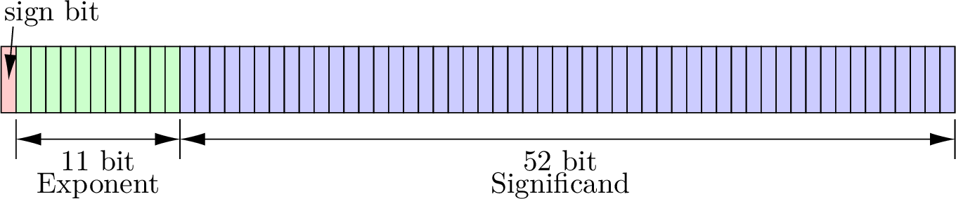
Fig. 6.23 The format of 64-bit double precision floating point numbers.
Let \(x_1 = mantissa_1 \times 2^{exponent_1}\) and let \(x_2 = mantissa_2 \times 2^{exponent_2}\). Further, let \(x_1\) be much greater than \(x_2\), (\(x_1 \gg x_2\)). The exponents are added in multiplication,
Division is a similar process, except the exponents are subtracted. Multiplication and division are immune to numerical problems except in the rare event of overflow or underflow.
Addition and subtraction require that the exponents match.
The expression \(\left(mantissa_2 \times 2^{(exponent_2 - exponent_1)}\right)\) where \(exponent_1 \gg exponent_2\), means that the binary digits of \(mantissa_2\) are shifted to the right \(exponent_1 - exponent_2\) positions. Any digits of \(mantissa_2\) that are shifted beyond the 52 positions of the significand are lost, and a round-off error is introduced into \(x_2\).
Many numbers have 1s in only a few positions to the right of the binary point. These numbers are not likely to lose precision to round-off error. But irrational numbers such as \(\pi\) or \(\sqrt{2}\) fill out the full 52 bits of the significand. They can suffer from a loss of precision with even a single-digit shift to the right due to adding a number that is only twice its value. Just as a fraction, such as \(1/3\), can hold infinitely repeating digits in decimal (\(0.333333 \ldots\)), some numbers have repeating digits in binary. For example, \((1.2)_{10} = (1.\underline{0011}0011\underline{0011}\ldots)_2\). A small round-off error occurs when a number as small as 2.4 is added to 1.2.
The example in figure Fig. 6.24 shows the round-off
error when 1.2 is added to successive powers of 2. When the variable
x is small, the variable y is close to zero. But as x gets
larger, variable a is increasingly lost to round-off error in
x + a, which causes variable y to converge to one. A logarithmic
scale on the \(y\) axis of the plot is needed to observe the loss of
precision. The stair-step shape to the plot is because a holds a
repeating pattern of the binary digits 0011. The precision of a is
diminished when a binary 1 is lost to round-off error. But no damage to
the precision of a occurs when a binary 0 is lost to round-off
error. The plot shows an interesting progression of the round-off error
when an irrational number is placed in the variable a. What do you
think the plot will look like when a simple number like 1.5 is placed in
a?
ex = 1:60;
x = 2.^ex;
a = 1.2;
y = abs(x + a - x - a)/a;
y(y < eps) = eps;
semilogy(ex, y)
axis tight
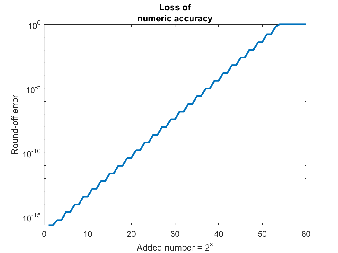
Fig. 6.24 The number a = 1.2 fills the full 52-bit significand allowed for double
precision floating point numbers. As the number added to a gets larger,
more of a is lost to round-off error.
6.9.2. Matrix Condition Number
Another problem besides round-off errors may degrade the accuracy of solutions to systems of equations. The symptom of the problem is an over-sensitivity to variations of the elements of \(\bm{b}\) when the system is nearly singular, which is also called poorly conditioned, or ill-conditioned. If the coefficients are taken from experiments, they likely contain a random component. We say there are perturbations to \(\bm{b}\). In many applications, \(\bf{A}\) is a fixed control matrix, so errors are more likely to be seen in \(\bm{b}\).
Errors in \(\bm{b}\), represented as \(\delta\bm{b}\), are conveyed to the solution \(\bm{x}\). The matrix equation \(\mathbf{A}\,\bm{x} = \bm{b}\) becomes \(\mathbf{A}\,\hat{\bm{x}} = \bm{b} + \delta\bm{b}\). Our estimate of the correct value of \(\bm{x}\) is \(\hat{\bm{x}} = \bm{x} + \bm{\delta x}\).
We care about the magnitudes of \(\bm{\delta x}\) and \(\bm{\delta b}\) relative to their true values. We want to find the length (norm) of each error vector relative to their unperturbed length, \(\norm{\bm{\delta x}} / \norm{\bm{x}}\) and \(\norm{\bm{\delta b}} / \norm{\bm{b}}\). We then have the following two inequalities because the norm of a product is less than or equal to the product of the norms of each variable.
Multiplying the two inequalities of equation (6.20) leads to equation (6.21).
Equation (6.21) defines the condition number of \(\mathbf{A}\), which is a metric that relates the error in \(\bm{x}\) to the error in \(\bm{b}\). The condition number measures how well or poorly conditioned a matrix is. The condition of \(\bf{A}\) is denoted as \(\kappa({\mathbf{A}})\) [WATKINS10].
Matrices that are close to singular have large condition numbers. If \(\kappa(\mathbf{A})\) is small, then small errors in \(\bm{b}\) results in only small errors in \(\bm{x}\). Whereas if \(\kappa(\mathbf{A})\) is large, then even small perturbations in \(\bm{b}\) can result in a large error in \(\bm{x}\). The condition number of the identity matrix and an orthogonal matrix is 1, but nearly singular matrices can have condition numbers of several thousand to even over a million.
The cond function in MATLAB uses the \(\norm{\cdot}_2\) matrix
norm by default, but may also compute the condition number using other
matrix norms defined in Matrix Norms. MATLAB calculates the
condition number using the singular values of the matrix as described in
Condition Number. Using the singular values, there is a concern about
division by zero, so MATLAB calculates the reciprocal, which it calls
RCOND. MATLAB’s left-divide operator checks the condition of a matrix
before attempting to find a solution. When using the left-divide
operator, one may occasionally see a warning message such as the
following:
Warning: Matrix is close to singular or badly scaled.Results may be inaccurate. RCOND = 3.700743e-18.
A handy rule of thumb for interpreting the condition number is if \(\kappa(\mathbf{A}) \approx 0.d \times 10^k\) then the solution \(\bm{x}\) can be expected to have \(k\) fewer digits of accuracy than the elements of \(\bf{A}\) [WILLIAMS14]. Thus, if \(\kappa(\mathbf{A}) = 10 = 0.1 \times 10^1\) and the elements of \(\bf{A}\) are given with six digits, then the solution in \(\bm{x}\) can be trusted to five digits of accuracy.
Here is an example to illustrate the problem. To be confident of the correct answer, we begin with a well-conditioned system.
It is easily confirmed with MATLAB that the solution is \(x_1 = -0.0621, x_2 = 0.9722\).
We assert that the system of equations in equation (6.23) is well-conditioned based on two pieces of information. First, the condition number of \(\bf{A}\) is a relatively small (2.3678). Secondly, minor changes to the equation have a minor impact on the solution. For example, if we add 1% of \(b_2\) to itself, we get a new solution of \(x_1 = -0.0609, x_2 = 0.9827\), which is a change of 2% to the solution \(x_1\) and 1.09% to \(x_2\).
Now, to illustrate a poorly conditioned system, we will alter the first equation of equation (6.23) to be the sum of the second equation and only \(1/100\) of itself.
Perhaps surprisingly, both LU decomposition and RREF can find the correct solution to equation (6.24). One can see that equation (6.24) is nearly singular because the two equations are close to parallel. The condition number is large (431). If we again add 1% of \(b_2\) to itself, we get a new solution of \(x_1 = -1.8617, x_2 = 0.1754\), which is a change to the \(x_1\) solution of 2,898%, and the \(x_2\) solution changed by 81.96%.
Another important result related to the condition number of matrices is that the condition number of the product of uncorrelated matrices is usually greater than the condition numbers of either of the individual matrices, and is sometimes equal to the product of the condition numbers of the individual matrices.
In the next section (Orthogonal Matrix Decompositions), we multiply orthogonal matrices without increasing the condition number of the product because the condition number of an orthogonal matrix is 1.
6.9.3. The Case for Partial Pivoting
For numerical stability, very small numbers should not be used as pivot variables in the elimination procedure. Each time the pivot is advanced, the remaining rows are sorted to maximize the absolute value of the pivot variable. The new row order is documented with a permutation matrix to associate results with their unknown variable. Reordering rows, or row exchanges, is also called partial pivoting. Full pivoting is when columns are also reordered.
Here is an example showing why partial pivoting is needed for numerical
stability. The example uses a \(2{\times}2\) matrix, where we could
see some round-off error. The \(\epsilon\) value used in the example
is taken to be a very small number, such as the machine epsilon value
(eps) that we used in
Example Control Constructs—sinc. Remember that round-off errors will propagate and build when solving a larger system of equations. Without pivoting, we divide potentially large numbers by \(\epsilon\), producing even larger numbers. In algebra, we can avoid large numbers but get small numbers in different places. In either case, during the row operation phase of elimination, we add or subtract numbers of very different values, resulting in round-off errors. The accumulated round-off errors become especially problematic in the substitution phase, where the denominator of a division might be near zero.
Regarding \(\epsilon\) as nearly zero relative to the other coefficients, we can use substitution to quickly see the approximate values of \(x_1\) and \(x_2\).
6.9.3.1. Elimination Without Partial Pivoting
If we don’t first exchange rows, we get the approximate value of \(x_2\) with some round-off error, but fail to find a correct value for \(x_1\).
Only one elimination step is needed.
We could multiply both sides of the equation by \(\epsilon\) to simplify it, or calculate the fractions. In either case, the 1 and 7 terms will be largely lost to round-off error.
Our calculation of \(x_1\) is completely wrong. Getting the correct answer requires dividing two numbers that are close to zero.
6.9.3.2. Elimination With Partial Pivoting
Now we begin with the rows exchanged.
Again, only one elimination step is needed.
We will again lose some accuracy to round-off errors, but our small \(\epsilon\) values are paired with larger values by addition or subtraction and have minimal impact on the back substitution equations.
MATLAB uses partial pivoting in both RREF and LU decomposition. It will use the small values in the calculation that we rounded to zero, so the results will be more accurate than our approximations.
>> x = A\b
x =
    3.0000
    2.0000
>> % not completely rounded
>> isequal(x, [3;2])
ans =
  logical
   0
6.9.4. The Case for LU Decomposition
Both MATLAB functions that use elimination (rref and lu) use
partial pivoting to improve the accuracy of the results. The rref
function is not as accurate as lu. Computer programs should use
lu to solve systems of equations. The use case for the rref
function is data analysis, exploration, and learning. However, rref
is accurate enough for most applications. Only very poorly conditioned
systems of equations will cause rref to fail to deliver reasonably
accurate results.
As a case study of what strategies achieve accurate results, we will
briefly consider some of the differences between the Gauss-Jordan
elimination algorithm used by rref and Turing’s kij LU decomposition
algorithm.
The kij LU algorithm has four noticeable differences from Gauss-Jordan elimination.
The pivot variables are not normalized to one before row operations. The pivot rows are not divided by the pivot variable.
Row operations are not used to move elements to the right of the diagonal to zero values. Rather, with the kij LU algorithm, the row operations directly yield both \(\bf{L}\) and \(\bf{U}\). Each row operation involves more additions or subtractions on the row elements, which is an additional opportunity to cause round-off errors.
Matrix elements below each pivot may never be set to zero from a row operation. The RREF row operations use subtraction to set matrix elements to zero. With the kij LU algorithm, the elements in \(\bf{U}\) below the diagonal are assigned a zero value. Assigning known values to variables is a certain step toward reducing round-off errors. If the math says that a variable should be zero or any other set value, then consider setting the variable to what it should be rather than relying on a mathematical operation to set it.
The corresponding values of the \(\bf{L}\) matrix are set by division, not subtraction.
The extra column of the \(\bm{b}\) vector is not a part of the elimination procedure. Although the \(\bm{b}\) vector is used in the LU algorithm’s forward and back substitution phases.
The second and third differences listed above likely contribute most to the less accurate results from Gauss-Jordan elimination than LU decomposition.
6.9.5. The Case for the Modified Gram–Schmidt Process
A comparison of the two Gram-Schmidt algorithms presented in Gram–Schmidt demonstrates the value of reordering addition or subtraction operations in favor of other operations in an algorithm such that the differences between the magnitudes of the two variables are minimized before addition or subtraction is performed.
Although currently used less than orthogonal factoring methods, such as the QR decomposition and the SVD, the classic Gram-Schmidt algorithm is an excellent application of vector projections. It is taught in many linear algebra courses. The objective is to find a set of orthogonal basis vectors from the columns of a matrix. In each step, the portion of a column that is not orthogonal to the columns to its right is subtracted away. The subtractions lead to an algorithm with poor numerical stability. The modified Gram–Schmidt (MGS) process offers better numerical stability to the classic Gram–Schmidt (CGS) process. From observations of the source code for the two functions, the key difference is when the subtractions occur. In the CGS process, the algorithm goes column by column, subtracting away the non-orthogonal components of each previous column. Then, after each column is orthogonal to the previous columns, it is normalized to a unit vector. In the MGS process, an outer loop goes down the diagonal of the matrix. The inner loop processes each sub-column below the current diagonal position. The sub-column is first scaled to a unit vector, then incremental subtractions remove the non-orthogonal components between unit vectors. Improved accuracy is achieved because, before each subtraction occurs, the two vectors involved have comparable magnitudes.
6.9.6. Lessons Learned
We have seen three case studies where improvements to algorithm design led to better numerical stability. Here we list a summary of strategies for algorithm design and programming practices that can improve the accuracy of calculations.
Avoid multiplication of large matrices. Remember that matrix multiplication involves sums of products, where round-off errors can accumulate. The condition number of matrices usually grows from matrix multiplication. The product \(\mathbf{A}^T\,\mathbf{A}\) becomes important to us for solving rectangular systems of equations and for finding the SVD factors in Singular Value Decomposition (SVD). [1]
Avoid division by numbers that are close to zero. When elimination is attempted without partial pivoting, problems occur when we divide by a number close to zero.
Less work is usually better. Use algorithms that perform fewer numeric operations on matrix elements. The additional row operations in the Gauss-Jordan procedure with the
rreffunction reduces the accuracy compared to the Gaussian elimination performed with LU decomposition.Let zero be zero. When the math equation says that a value after a certain operation should be zero. Then, make an assignment statement to set it to zero or whatever known quantity the math says it should be. The numeric operation performed by the computer will likely not set it to exactly zero due to round-off errors. To convince yourself that this simple step improves the accuracy of results, try informal experiments with factoring algorithms such as LU and QR ( QR Decomposition) decomposition.
Order the steps of algorithms such that when two numbers are added together or subtracted from each other, the numbers are close to the same value. The modified Gram-Schmidt process improves numerical accuracy by only subtracting unit-length vectors.
Footnote
