13.2. Vector Spaces

Here we will define some linear algebra terms and explain some foundational concepts related to vector spaces, dimension, linearly independent vectors, and rank.

Vector Space

A vector space consists of a set of vectors and scalars that is closed under vector addition and scalar multiplication.

Saying that a vector space is closed means we can add any vectors from the set together and multiply vectors by scalars, and the resulting vectors are still in the vector space.

For example, vectors in 3 dimensions are said to be in a vector space called \(\mathbb{R}^3\). If the basis vectors of the space are the standard orthogonal coordinate frame, then the set of vectors in \(\mathbb{R}^3\) consists of three real numbers defining their magnitude in the \(\bm{x}\), \(\bm{y}\), and \(\bm{z}\) directions.

Span

The set of all linear combinations of a collection of vectors is called the span of the vectors. If a vector can be expressed as a linear combination of a set of vectors, then the vector is in the span of the set.

Basis

The smallest set of vectors needed to span a vector space forms a basis for that vector space.

The vectors in the vector space are linear combinations of the basis vectors. For example, the basis vectors used for a Cartesian coordinate frame in the vector space \(\mathbb{R}^3\) are:

\[\begin{split}\left\{ \begin{bmatrix} 1 \\ 0 \\ 0 \end{bmatrix}, \; \begin{bmatrix} 0 \\ 1 \\ 0 \end{bmatrix}, \; \begin{bmatrix} 0 \\ 0 \\ 1 \end{bmatrix} \right\}\end{split}\]

Many different basis vectors could be used as long as they are a linearly independent set of vectors, but we prefer unit-length orthogonal vectors. In addition to the Cartesian coordinates, other sets of basis vectors are sometimes used. For example, some manufacturing applications may use basis vectors that span a plane corresponding to a workpiece. Other applications, such as difference equations, use the set of eigenvectors of a matrix as the basis vectors.

Dimension

The number of basis vectors of a vector space is its dimension.

For the Cartesian basis vectors, \(\mathbb{R}^3\) and \(\mathbb{R}^2\), the dimension is the number of elements in the vectors. However, other vector spaces may have a smaller dimension. For example, the subspace where the \(z\) axis is the same as the \(x\) axis (\(z = x\)) forms a plane with dimension 2, which is plotted in figure Fig. 13.2. The orthonormal basis vectors for this subspace might be

\[\begin{split}\left\{ \bm{v}_1, \bm{v}_2 \right\} = \left\{ \frac{1}{\sqrt{2}}\,\begin{bmatrix} 1 \\ 0 \\ 1 \end{bmatrix}, \begin{bmatrix} 0 \\ 1 \\ 0 \end{bmatrix} \right\}.\end{split}\]

We may reference points or vectors in a subspace with two dimensions, \((a, b)\). Linear combinations of the basis vectors are used to find the coordinates of the point in the \(\mathbb{R}^3\) world.

\[\begin{split}\begin{bmatrix} a \\ b \end{bmatrix} \longmapsto a\,\bm{v}_1 + b\,\bm{v}_2\end{split}\]

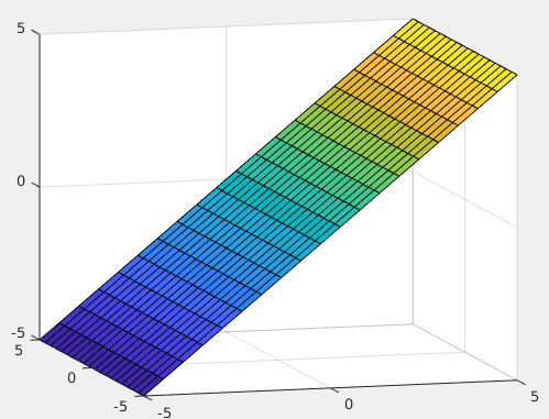
Fig. 13.2 Vector space where \(z = x\), dimension = 2.

Linearly Independent Vectors

The set of vectors, \({\bm{u}_1, \bm{u}_2, \ldots \bm{u}_n}\), are linearly independent if for any scalars \(c_1, c_2, \ldots c_n\), the equation \(c_1\,\bm{u}_1 + c_2\,\bm{u}_2 + \cdots + c_n\,\bm{u}_n = 0\) has only the solution \(c_1 = c_2 = \cdots = c_n = 0\).

The official definition of linearly independent vectors may at first seem a bit obscure, but it is worth stating along with some explanation and examples.

A set of vectors is linearly independent if no vector in the set is a linear combination of the other vectors. If a linear combination of other vectors can find one or more vectors in the set, the vectors are not linearly independent. There are nonzero coefficients, \(c_i\), that will satisfy the equation \(c_1\,\bm{u}_1 + c_2\,\bm{u}_2 + \ldots + c_n\,\bm{u}_n = 0\).

For example, the basis vectors used for a Cartesian coordinate frame in the vector space \(\mathbb{R}^3\) are linearly independent.

\[\begin{split}\left\{ \begin{bmatrix} 1 \\ 0 \\ 0 \end{bmatrix}, \; \begin{bmatrix} 0 \\ 1 \\ 0 \end{bmatrix}, \; \begin{bmatrix} 0 \\ 0 \\ 1 \end{bmatrix} \right\}\end{split}\]

Whereas, the following set of vectors is not linearly independent because the last vector is the sum of the first two vectors, thus \(\bm{u}_1 + \bm{u}_2 - \bm{u}_3 = \bm{0}\).

\[\begin{split}\left\{ \begin{bmatrix} 1 \\ 0 \\ 1 \end{bmatrix}, \; \begin{bmatrix} 0 \\ 1 \\ 0 \end{bmatrix}, \; \begin{bmatrix} 1 \\ 1 \\ 1 \end{bmatrix} \right\}\end{split}\]

When we evaluate the columns of a matrix, \(\bf{A}\), with regard to another vector, \(\bm{b}\), we might say that vector \(\bm{b}\) is in the column space of \(\bf{A}\), which means that \(\bf{b}\) is a linear combination of the vectors that define the columns of matrix \(\bf{A}\).

Rank

The rank of a matrix is the maximum number of linearly independent rows or columns in the matrix.

Two different methods can determine the rank of a matrix. The rank of a matrix is the number of nonzero pivots in its row-echelon form, which is achieved by Gaussian elimination. Here is an example illustrating how elimination on a singular matrix results in a pivot value equal to zero. Because of dependent relationships between the rows and columns, the row operations to change elements below the diagonal to zeros also move the later pivots to zero. In this example, the third column is the sum of the first column and two times the second column.

\[\begin{split}\begin{bmatrix} \underline{3} & 2 & 7 \\ 0 & 3 & 6 \\ 1 & 0 & 1 \end{bmatrix}\end{split}\]

Add \(-1/3\) of row 1 to row 3. The pivot then moves to row 2.

\[\begin{split}\begin{bmatrix} 3 & 2 & 7 \\ 0 & \underline{3} & 6 \\ 0 & -2/3 & -4/3 \end{bmatrix}\end{split}\]

Add \(2/9\) of row 2 to row 3.

\[\begin{split}\begin{bmatrix} 3 & 2 & 7 \\ 0 & 3 & 6 \\ 0 & 0 & 0 \end{bmatrix}\end{split}\]

Thus, with two nonzero pivots, the rank of the matrix is 2.

The second method for computing rank is to use the singular value decomposition (SVD) as demonstrated in Rank from the SVD. The number of singular values above a small tolerance is the rank of the matrix. The MATLAB rank function uses the SVD method.