9.5. Fundamental Matrix Subspaces
There are four fundamental subspaces of an \(m{\times}n\) matrix. The subspaces are found from rank-determined regions of the SVD factors. The regions are identified in figure Fig. 9.6 as the Column Space (\(\mathbf{\tilde{U}}\)), Left Null Space (\(\mathbf{U}_{null}\)), Row Space (\(\mathbf{\tilde{V}}^T\)), and Null Space (\(\mathbf{V}_{null}^T\)).
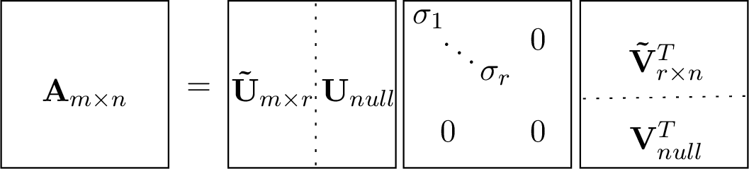
Fig. 9.6 The columns of \(\bf{U}\) and rows of \(\mathbf{V}^T\) from the SVD constitute the four fundamental matrix subspaces of the matrix. The subspace that a row or column is part of is determined by whether it is multiplied by a nonzero or zero singular value.
If we consider the SVD of a singular system as \(\mathbf{A\, V} = \mathbf{U\,\Sigma}\), then we can divide the \(\bf{V}\), \(\bf{\Sigma}\), and \(\bf{U}\) matrices into blocks related to the nonzero and zero-valued singular values.
9.5.1. Column Space
The column space (\(\mathbf{\tilde{U}}\)) of a matrix \(\bf{A}\), which we denote as \(\text{Col}( \bf{A} )\), is the vector space spanned by the independent columns of \(\bf{A}\). It is the first \(r\) columns of \(\bf{U}\), and includes all columns of \(\bf{U}\) if \(\bf{A}\) is square and full rank. The column space from \(\bf{U}\) forms a set of basis vectors for the columns of \(\bf{A}\). However, Finding Orthogonal Basis Vectors lists other algorithms for finding orthogonal basis vectors.
When there is an exact solution to the equation \(\mathbf{A}\,\bm{x} = \bm{b}\), we say that \(\bm{b}\) is “in the column space of \(\bf{A}\)” because it is a linear combination of the independent columns of \(\bf{A}\). Similarly, the columns of \(\bf{A}\) are linear combinations of the columns of \(\text{Col}( \mathbf{A} )\). Note that when \(\bf{A}\) is square and full rank, all singular values are non-zero, making \(\bf{A}\) invertible and guaranteeing that the column space of \(\bf{A}\) spans the entire \(\mathbb{R}^n\) space. Thus, all of the columns of \(\mathbf{U}\) form \(\text{Col}( \bf{A} )\) for square, full rank matrices. We can verify that \(\mathbf{\tilde{U}}\) forms \(\text{Col}( \bf{A} )\) with two tests when \(\bf{A}\) is singular or over-determined. The columns of \(\mathbf{\tilde{U}}\) and \(\bf{A}\) are in the same vector space if the rank of the augmented matrix \([\mathbf{\tilde{U} \, A}]\) and \(\bf{A}\) is the same. \(\mathbf{\tilde{U}}\) is a basis for \(\text{Col}( \mathbf{A} )\) when the projection of \(\bf{A}\) onto \(\mathbf{\tilde{U}}\) yields \(\bf{A}\).
Here is a singular matrix example showing that \(\mathbf{\tilde{U}}\) forms \(\text{Col}( \mathbf{A} )\). We will use the alternate projection equation from Alternate Projection Equation.
>> % A is random 3-by-3
>> A(:,3)=-2*A(:,1)-A(:,2);
>> rank(A)
ans =
    2
>> [U, ~, ~] = svd(A);
>> rank([U(:,1:2) A(:,1:2)])
ans =
     2
9.5.2. Null Space
Columns \(r+1\) to \(n\) of \(\mathbf{V}\) form the null
space (right null space) (\(\mathbf{V}_{null}^T\) in figure
Fig. 9.6) of a matrix \(\bf{A}\), which we
denote as \(\text{Null}( \bf{A} )\). It is the vector space spanned
by all column vectors \(\bm{x}\) that satisfy the matrix equation
\(\mathbf{A}\,\bm{x} = \bm{0}\), which is called the null solution.
As mentioned in The Row and Column View, the only square systems with a
null solution are singular. Singular square matrices and
under-determined matrices have a null space. The number of vectors in
the null space is the number of dependent columns
(size(A, 2) - rank(A)). If \(\bf{A}\) is a square full-rank
matrix, then the null space is an empty set.
Finding the null space from elimination is covered in
Finding Eigenvectors. But MATLAB’s null function returns the null
space from the SVD.
Null space from the SVD
Theorem 9.3 (Null space from the SVD)
Let \(\mathbf{A} \in \mathbb{R}^{n{\times}n}\) be singular with \(r = \text{rank}(\mathbf{A}) < n\). Each of the last \(n-r\) columns of \(\bf{V}\) are null solutions of \(\bf{A}\), \(\mathbf{A}\,\bm{v}_i = \bm{0}\).
Proof. Let the SVD of a singular system be \(\mathbf{A\, V} = \mathbf{U\,\Sigma}\). As equation (9.2) shows, we can split the \(\bf{V}\), \(\bf{\Sigma}\), and \(\bf{U}\) matrices into blocks related to nonzero and zero-valued singular values.
The last \(n - r\) columns of \(\bf{V}\) is the null solution because \(\mathbf{A}\,\mathbf{V}_{null} = \mathbf{0}\).
\(\qed\)
MATLAB’s null function compares the singular values to a threshold
to decide if and how many columns of \(\bf{V}\) constitute the null
space. However, determining if a matrix is singular, or just close to
singular, is sometimes vague. The null function will sometimes not
return a solution for nearly singular matrices. In these cases, the SVD
can be used to find the borderline null solution.
>> % A is 3-by-3
>> % rank(A) = 2
>> [~,~,V] = svd(A);
>> x = V(:,3); % = null(A)
>> A*x
ans =
     0
     0
     0
The null space of an under-determined matrix is at least (\(m-n\)) columns. Remember from Under-determined Systems that under-determined systems have an infinite number of solutions. The RREF expresses the solution in terms of the general and particular solutions, while the null space from the SVD is the least squares solution. Although the solutions are different, they are both correct.
>> A = randi(20, 3, 5) - 8;
>> [~, ~, V] = svd(A);
>> r = rank(A);
>> nullA = V(:, r+1:end);
>> A*nullA
ans =
   1.0e-14 *
   -0.0583    0.0992
    0.0444   -0.0666
   -0.0722   -0.1568
9.5.3. Row Space
The row space (\(\mathbf{\tilde{V}}^T\)) of a matrix \(\bf{A}\), which we denote as \(\text{Row}( \bf{A} )\), is the column space of \(\mathbf{A}^T\). It is the first \(r\) columns of \(\bf{V}\) from the SVD.
9.5.4. Left Null Space
The left null space (\(\mathbf{U}_{null}\)) of a matrix
\(\bf{A}\) are the set of row vectors, \(\bf{Y}\), that satisfy
the relationship \(\bf{Y\,A} = \bm{0}\). It is the transpose of
columns \(r+1\) to \(m\) of \(\bf{U}\). It is also the right
null space of \(\mathbf{A}^T\), and it is common to compute it from
\(\mathbf{A}^T\), Y = null(A’)’. The left null space exists for
singular and over-determined matrices.
9.5.5. Orthogonality of Spaces
The four fundamental vector subspaces form interesting orthogonality relationships, which is expected since they are subsets of the orthogonal matrices \(\bf{U}\) and \(\bf{V}\). Vectors in the null space are orthogonal to vectors in the row space. Similarly, vectors in the column space are orthogonal to vectors in the left null space.
