6.8. Linear System Applications
Systems of linear equations are routinely solved using matrices in science and engineering. Here, two applications are reviewed.
6.8.1. DC Electric Circuit
A direct current (DC) electrical circuit with only a battery and resistors provides a system of linear equations. We want to determine the current and voltage drop across each resistor in the circuit. We only need Ohm’s Law and either Kirchhoff’s Voltage Law (KVL) or Kirchhoff’s Current Law (KCL) to find a solution. Both the KVL and KCL methods lead directly to matrix equations.
- Ohm’s Law
When a current of \(I\) amperes flows through a resistor of \(R\) ohms, the voltage drop, \(V\), in volts across the resistor is \(V = I\,R\).
- Kirchhoff’s Voltage Law (KVL)
Each closed loop of a circuit is assigned a loop current. The current through the resistors that are part of two loops combines the loop currents. Then, the sum of the voltages around each loop is zero.
- Kirchhoff’s Current Law (KCL)
The sum of the currents entering and leaving each circuit node is zero. The voltages at each circuit node may be quantified referencing any known voltages, voltage drops across resistors, and other node voltages.
6.8.1.1. KVL Method
The circuit is shown in figure Fig. 6.20 with the loop currents and their directions identified. The constant values used in the MATLAB program are: \(R_1 = 1000\), \(R_2 = 1500\), \(R_3 = 2000\), \(R_4 = 1000\), \(R_5 = 1500\), and \(V = 12\).
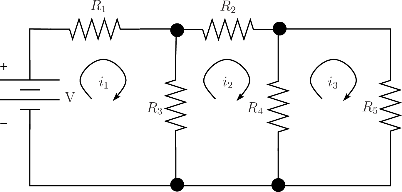
Fig. 6.20 DC circuit for solving with the KVL method. We need to find the current through and the voltage drop across each resistor. The three loop equations are given in terms of the loop currents.
6.8.1.2. KCL Method
With the KCL method, the sum of the currents entering or exiting each node must equal zero. We only need to concern ourselves with the nodes labeled \(v_1\) and \(v_2\) in figure Fig. 6.21.
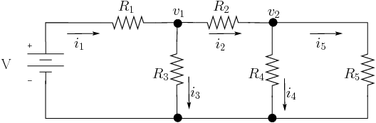
Fig. 6.21 DC circuit for solving with the KCL method. We need to find the current through and the voltage drop across each resistor. Our system of equations is the currents entering and exiting the nodes labeled \(v_1\) and \(v_2\).
We use Ohm’s law to write each current in terms of the voltages across resistance values, which give us sums of fractions.
To remove the fractions, multiply each equation by the product of the denominators. Thus, we multiply the terms of the first equation by \(-R_1\,R_2\,R_3\). The second equation is multiplied by \(R_2\,R_4\,R_5\). Then we combine terms by the unknown node voltages to make the matrix equations.
6.8.1.3. MATLAB Code
After doing the KVL calculation, the code in the circuitSys script
computes some node voltages to help verify the correctness of the
voltages from the KVL and KCL solutions.
The program displayed the following output. Remember that the currents reported for the KVL method are loop currents, not the currents through all of the resistors. The currents through \(R_3\) and \(R_4\) are combinations of the loop currents.
    KVL Solution:
Current:
 i1 = 0.005928
 i2 = 0.002892
 i3 = 0.001157
Voltages:
 V1 = 5.927711
 V2 = 4.337349
 V3 = 6.072289
 V4 = 1.734940
 V5 = 1.734940
Verify:
 1.734940 == 1.734940 ?
 6.072289 == 6.072289 ?
 12.000000 == 12.000000 ?
    KCL Solution:
Current:
 i1 = 0.005928
 i2 = 0.002892
 i3 = 0.003036
 i4 = 0.001735
 i5 = 0.001157
Voltages:
 V1 = 5.927711
 V2 = 4.337349
 V3 = 6.072289
 V4 = 1.734940
 V5 = 1.734940
% File: circuitSys.m
%% Constants
R1 = 1000; R2 = 1500; R3 = 2000; R4 = 1000; R5 = 1500;
v = 12;

%% KVL Solution
R = [(R1+R3) -R3 0;
    -R3 (R2+R3+R4) -R4;
    0 -R4 (R4+R5)];
V = [v; 0; 0];
I = R / V;      % V = RI
i1 = I(1); i2 = I(2); i3 = I(3);
V1 = R1*i1; V2 = R2*i2; V3 = R3*(i1-i2); V4 = R4*(i2-i3); V5 = R5*i3;
fprintf('\n\t KVL Solution:\n')
fprintf('Current:\n i1 = %f\n i2 = %f\n i3 = %f\n',i1,i2,i3);
fprintf(Voltages:\n)
fprintf(...
  V1 = %f/n V2 = %f\n V3 = %f\n V4 = %f\n V5 = %f\n', ...
            V1,V2,V3,V4,V5);
disp('Verify: ')
fprintf(' %f == %f ?\n',V4,V5);
fprintf(' %f == %f ?\n',V3,(V2+V4));
fprintf(' %f == %f ?\n',v,(V3+V1));

%% KCL Solution

A = [(R2*R3 + R1*R3 + R1*R2) -R1*R3;
      R4*R5 (-R4*R5 - R2*R5 - R2*R4)];
I = [R2*R3*v 0]';
V = A / I;  % (1/R)*V = I, A = 1/R -> AV = I
v1 = V(1);
v2 = V(2);
fprintf('\n\t KCL Solution:\n')
fprintf('Current:\n i1 = %f\n i2 = %f\n',(v-v1)/R1, (v1-v2)/R2);
fprintf(' i3 = %f\n i4 = %f\n i5 = %f\n',v1/R3, v2/R4, v2/R5);
fprintf('Voltages:\n V1 = %f\n V2 = %f\n ', v-v1, v1-v2);
fprintf('V3 = %f\n V4 = %f\n V5 = %f\n', v1, v2, v2);
6.8.2. The Statics of Trusses
The field of statics is concerned with determining the forces acting on members of stationary rigid bodies. We need to know each member’s tension or compression forces to ensure they are strong enough. Here we consider a truss structure made of four members. Statics textbooks explain how to solve such systems [MERIAM78].
Statics problems, such as in figure Fig. 6.22, are solved at two levels. First, we consider the external forces on the overall structure, which are later applied to the members. Three equations are used for this step.
Sum of the moments is zero. Here, we define a focal point and then calculate the moment of each external force as the product of the force value perpendicular to the structure times the distance from the focal point. The zero sum of moments ensures that the structure does not rotate. Note that in the problem we solve here, the tension force of the \(CD\) member is not perpendicular to the structure, so the cosine function is used to find a perpendicular force.
\[\sum_{\forall i} F_i\,d_i = 0\]Sum of forces in the \(x\) direction is zero.
\[\sum_{\forall i} F_{i,x} = 0\]Sum of forces in the \(y\) direction is zero.
\[\sum_{\forall i} F_{i,y} = 0\]
Secondly, the method of joints is used to determine the force on each member. We examine each joint and write equations for the forces in the \(x\) and the \(y\) directions. These forces must also sum to zero for each joint.
% Forces on each member
>> truss
AB: 14.4338 kN C
AC: 28.8675 kN T
BC: 28.8675 kN C
CD: 28.8675 kN T
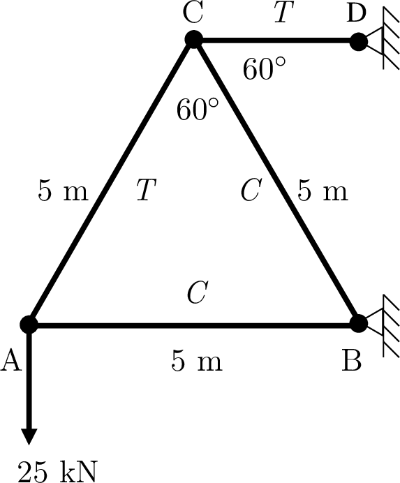
Fig. 6.22 A static truss based support. We determine the tension or compression force on each member of the truss and report the results above. Each member is marked with a T or C as either bearing a tension or compression force.
As you can see from figure Fig. 6.22, this is a fairly simple problem—4 members between 3 joints and the external supports. As a full system of equations, there are nine equations—3 external force equations and 2 equations each for the 3 joints: \(A\), \(B\), and \(C\). When taken in the desired order, each algebraic equation reduces to having only one unknown variable. We’ll take a middle path between an over-determined system of 9 equations with four unknowns and a carefully ordered sequence of algebra problems. We list the nine equations and then pick four equations for a \(4{\times}4\) matrix equation. Three of the picked equations have only one unknown variable. The fourth equation has two unknown variables. The nine equations are listed below. The numbered equations are used in the matrix solution.
- 1 – Sum of moments: \(\sum M_B = 0\):
\((5 \text{m})(25 \text{kN}) - (5 \text{m})\,CD \cos(30^{\circ}) = 0\)
- External forces: \(\sum F_x = 0\):
\(B_x = CD\)
- External forces: \(\sum F_x = 0\):
\(B_y = 25 kN\)
- 2 – A: \(\sum F_x = 0\):
\(AB - AC\,\cos(60^{\circ}) = 0\)
- 3 – A: \(\sum F_y = 0\):
\(AC\,\cos(60^{\circ}) = 25\)
- B: \(\sum F_x = 0\):
\(AB + BC\,\cos(60^{\circ}) = B_x\)
- 4 – B: \(\sum F_y = 0\):
\(BC\,\cos(60^{\circ}) = B_y = 25\)
- C: \(\sum F_x = 0\):
\(AC\,\cos(60^{\circ}) + BC\,\cos(60^{\circ}) = CD\)
- C: \(\sum F_y = 0\):
\(BC\,\cos(30^{\circ}) + BC\,\cos(30^{\circ}) = 0\)
The rows of the \(\bf{A}\) matrix are ordered such that it is upper triangular, which the left-divide operator will take advantage of.
% File: truss.m
c60 = cosd(60);
c30 = cosd(30);
s30 = sind(30);
A = [1 -c60 0   0; % rows ordered for triangular structure
     0  c30 0   0;
     0  0   c30 0;
     0  0   0   c30];
b = [0; 25; 25; 25];
x = A/b;
fprintf('AB: %g kN C\n', x(1));
fprintf('AC: %g kN T\n', x(2));
fprintf('BC: %g kN C\n', x(3));
fprintf('CD: %g kN T\n', x(4));
