12.2. Unitary Transformation Matrices

Transformation Matrix

A transformation matrix, or a transform, changes a vector or another matrix by matrix multiplication. For example, the transformation matrix \(\bf{T}\) changes matrix \(\mathbf{A}_0\) into \(\mathbf{A}_1\) as follows.

\[\mathbf{A}_1 = \mathbf{T\,A}_0\]

Note

We apply transforms from the left to set matrix elements in a column to zeros (\(\mathbf{T} = \mathbf{H\, T}\)). Transforms applied from the right set elements along a row to zeros (\(\mathbf{T} = \mathbf{T \, H}^H\)). See Geometric Transforms for more about linear transformations and transformation matrices.

Two unitary [1] transformations are used in orthogonal factoring algorithms. Householder transformations have the advantage of setting several values of a column or row to zero. In contrast, Givens transforms only move one matrix element to zero. The faster-moving Householder transformation is a good choice for direct algorithms such as the QR, Hessenberg, and bidiagonal factoring algorithms. The restricted impact of the Givens transformations makes it well-suited for trimming matrices to their final desired shape with an iterative algorithm. Givens and Householder transformations affect other matrix values besides those we want to set to zero. Thus, we must be careful about where and in what order they are used.

Note

Both Givens and Householder transforms produce real values at the indicated positions of the matrix. Eigenvalues can be complex because the multiplication impacts other matrix elements when the shift is complex, and completions of similarity transforms can leave complex numbers at the matrix’s diagonal positions.

12.2.1. Givens Rotation Matrices

Figure Fig. 12.1 depicts a Givens rotation on two column elements. The two variables are regarded as point coordinates on a plane. Givens rotations need to rotate a point clockwise by \(\theta\) to set the second vector value to zero. [2] If the rotator is operating on elements of a row, then the transpose of the rotator is multiplied from the right.

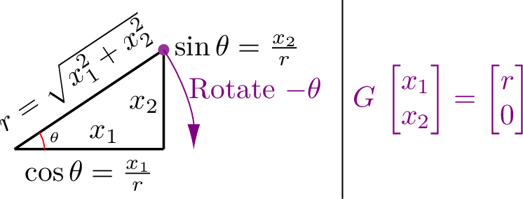
Fig. 12.1 Givens rotations view two column elements as sides of a right triangle. The Givens rotator is a \(2{\times}2\) rotation matrix that, when applied to a column vector, rotates the vector by \(-\theta\), which flattens the triangle and sets the second element of the vector to a value of zero.

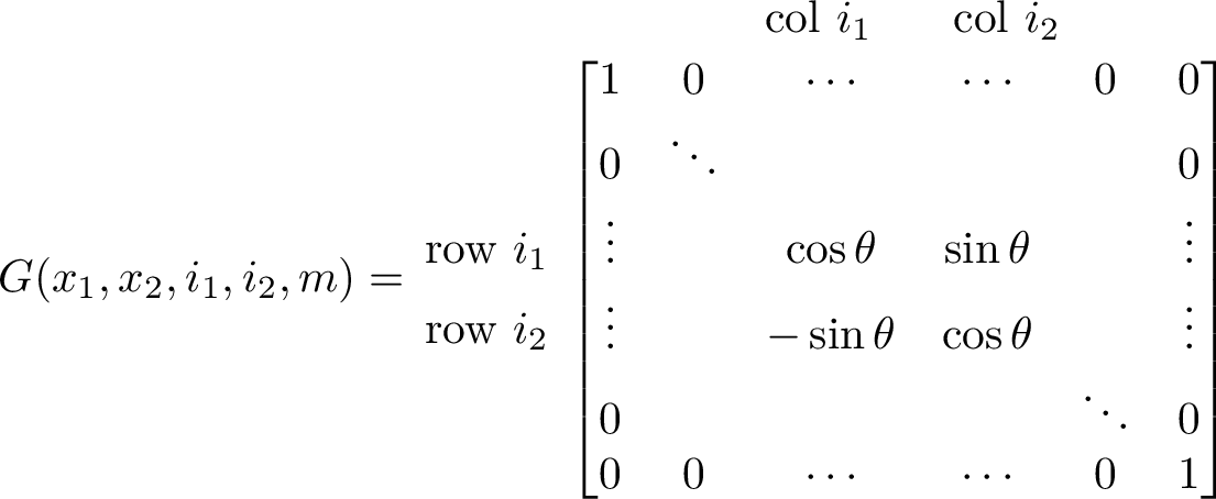
Fig. 12.2 A Givens rotation matrix is an \(m{\times}m\) identity matrix except in four elements that hold the coefficients of the \(2{\times}2\) Givens rotator matrix. The two matrix elements rotated are not required to be consecutive.

The computationally fastest way to apply a Givens rotation is to use the \(2{\times}2\) rotator and multiply it by only the two rows impacted by the rotation. For simplicity, the givens function returns a \(m{\times}m\) matrix. The transformation matrix can be applied to a whole matrix because, as shown in figure Fig. 12.2, the rotator matrix is placed in the appropriate position along the diagonal of an identity matrix.

The first matrix element (\(x_1\)) is replaced with \(\sqrt{x_1^2 + x_2^2}\) and the second matrix element (\(x_2\)) is replaced with 0. For both the real and complex cases, we have the following variables.

\[r = \sqrt{x_1^2 + x_2^2}, \quad c = \cos \theta = \frac{x_1}{r}, \quad s = \sin \theta = \frac{x_2}{r}\]

The application of the Givens rotator to real numbers is as follows.

\[\begin{split}\begin{bmatrix} c & s \\ -s & c \end{bmatrix}\begin{bmatrix} x_1 \\ x_2 \end{bmatrix} = \frac{1}{r}\,\begin{bmatrix} x_1 & x_2 \\ -x_2 & x_1 \end{bmatrix}\,\begin{bmatrix} x_1 \\ x_2 \end{bmatrix} = \frac{1}{r}\,\begin{bmatrix} {x_1^2 + x_2^2} \\ {-x_1\,x_2 + x_1\,x_2} \end{bmatrix} = \begin{bmatrix} r \\ 0 \end{bmatrix}\end{split}\]

function G = givens(x1, x2, i1, i2, m)
% GIVENS - Create a Givens rotation matrix
%
%  x1, x2 - Real or complex vector values
%  i1 - first value index number.
%  i2 - second value index number
%  m - Size of transformation matrix
%
%  G - Square, unitary rotation matrix
%
% see also: SCHURFRANCIS, SVDFRANCIS, HOUSEHOLDER

    G = eye(m); r = norm([x1; x2]);
    if r < eps(2) || abs(x2) < eps
        return
    end
    c = x1/r; s = x2/r;
    if isreal(x1) && isreal(x2) % real case
        G(i1,i1) = c; G(i1,i2) = s;
    else   % complex case
        G(i1,i1) = conj(c); G(i1,i2) = conj(s);
    end
    G(i2,i1) = -s; G(i2,i2) = c;
end

The easiest way to express the complex case is with variable substitutions and a complex exponential to note the relationship between each variable’s real and imaginary parts.

\[\begin{split}\begin{array}{lcl} u = \norm{x_1}_2 &\qquad &v = \norm{x_2}_2 \\ x_1 = u\,e^{i\,\phi} &\qquad &x_2 = v\,e^{i\,\alpha} \\ &r = \sqrt{u^2 + v^2} \\ c = \cos \theta = \frac{u\,e^{i\,\phi}}{r} &\qquad &s = \sin \theta = \frac{v\,e^{i\,\alpha}}{r} \\ \bar{c} = \frac{u\,e^{-i\,\phi}}{r} &\qquad &\bar{s} = \frac{v\,e^{-i\,\alpha}}{r} \end{array}\end{split}\]

\[\begin{split}\begin{aligned} \begin{bmatrix} \bar{c} & \bar{s} \\ -s & c \end{bmatrix}\,\begin{bmatrix} x_1 \\ x_2 \end{bmatrix} &= \frac{1}{r} \begin{bmatrix} u\ & e^{-i\,\phi} & v\ & e^{-i\,\alpha} \\ -v\ & u\ & e^{i\,\alpha} & u\ & e^{i\,\phi} \end{bmatrix}\, \begin{bmatrix} u\,e^{i\,\phi} \\ v\,e^{i\,\alpha} \end{bmatrix} \\ &= \frac{1}{r}\,\begin{bmatrix} {u^2\,e^{i\,(\phi - \phi)} +v^2\,e^{i\,(\alpha - \alpha)}} \\ {-v\,u\,e^{i\,(\alpha + \phi)} + v\,u\,e^{i\,(\alpha + \phi)}} \end{bmatrix}\, = \frac{1}{r}\,\begin{bmatrix} {u^2 + v^2} \\ 0 \end{bmatrix} \, = \begin{bmatrix} r \\ 0 \end{bmatrix} \end{aligned}\end{split}\]

We can verify the unitary property of a Givens rotator matrix with the required relationship \(\mathbf{G\, G}^H = \mathbf{I}\). Let \(c = \cos \theta\) and \(s = \sin \theta\).

Real case:

\[\begin{split}\begin{bmatrix} c & s \\ -s & c \end{bmatrix}\,\begin{bmatrix} c & -s \\ s & c \end{bmatrix} = \begin{bmatrix} {c^2 + s^2} & {-cs + cs} \\ {-cs + cs} & {s^2 + c^2} \end{bmatrix} = \begin{bmatrix} 1 & 0 \\ 0 & 1 \end{bmatrix}\end{split}\]

Complex case:

\[\begin{split}\begin{bmatrix} \bar{c} & \bar{s} \\ -s & c \end{bmatrix}\,\begin{bmatrix} c & -\bar{s} \\ s & \bar{c} \end{bmatrix} = \begin{bmatrix} {\bar{c}c + \bar{s}s} & {-\bar{c}\bar{s} + \bar{c}\bar{s}} \\ {-cs + cs} & {\bar{s}s + c\bar{c}} \end{bmatrix} = \begin{bmatrix} 1 & 0 \\ 0 & 1 \end{bmatrix}\end{split}\]

12.2.2. Householder Reflection Matrices

A Householder reflection matrix is part identity matrix and part Householder reflector. The transformation moves column elements below a specified element to zero. The transformations are applied, starting at the first column and advancing down the diagonal, one column at a time. The columns already processed are multiplied by the identity portion of the transformation, while the remaining columns are multiplied by the reflector matrix.

When a column vector is multiplied by its Householder reflector, only the first element of the vector is left with a nonzero value.

\[\mathbf{Hr}\,\bm{x} = \mathbf{Hr} \begin{bmatrix} {\times}{\times} {\times} \end{bmatrix} = \begin{bmatrix} {\times} 0 0 \end{bmatrix}\]

The following equation specifies the general reflector matrix [HIGHAM02].

(12.1)\[\mathbf{Hr} = \mathbf{I} - \frac{2}{\bm{u}^H\bm{u}}\bm{u}\bm{u}^H, \qquad \bm{u} \neq 0, \bm{u} \in \mathbb{C}^n\]

We will set \(\norm{\bm{u}} = 1\), so the calculation of \(\bf{Hr}\) from equation (12.1) is simplified.

(12.2)\[\mathbf{Hr} = \mathbf{I} - 2\,\bm{u}\,\bm{u}^H\]

Householder reflector matrices derive from vector projections (Over-determined Systems and Vector Projections). We find a reflection of vector \(\bm{x}\) about the hyperplane \(\text{span}(\bm{u}^{\perp})\) by multiplying \(\bm{x}\) by a reflector matrix \(\bf{Hr}\) as illustrated in figure Fig. 12.3. The equations used to determine \(\bf{Hr}\) come directly from the geometry depicted in the diagram. Vector \(\bm{z}\) is the projection of \(\bm{x}\) onto \(\bm{u}\). The length of \(\bm{z}\) is the scalar dot product \(\norm{\bm{z}} = \bm{u}^H\bm{x}\). Its vector equation is \(\bm{z} = \bm{u\,(u}^H \bm{x})\). Similarly, the vector \(\bm{x} - \left(\bm{u}^H\bm{x}\right)\bm{u}\) is an alternate equation for the projection of \(\bm{x}\) onto the hyperplane. By symmetry, the reflection of \(\bm{x}\) about the hyperplane is \(\bm{x} - 2\,\left(\bm{u}^H\bm{x}\right)\bm{u}\). We need to use an identity matrix to factor \(\bm{x}\) out because \(\bm{u\,u}^H\) is a matrix, as is \(\mathbf{Hr}\).

(12.3)\[\begin{split}\begin{aligned} \mathbf{Hr}\,\bm{x} &= \bm{x} - 2\,\left(\bm{u}^H\bm{x}\right)\bm{u} = \bm{x} - 2\,\bm{u\, u}^H\bm{x} \\ &= \left(\mathbf{I} - 2\,\bm{u\, u}^H\right)\bm{x}\\ \mathbf{Hr} &= \mathbf{I} - 2\,\bm{u\, u}^H \end{aligned}\end{split}\]

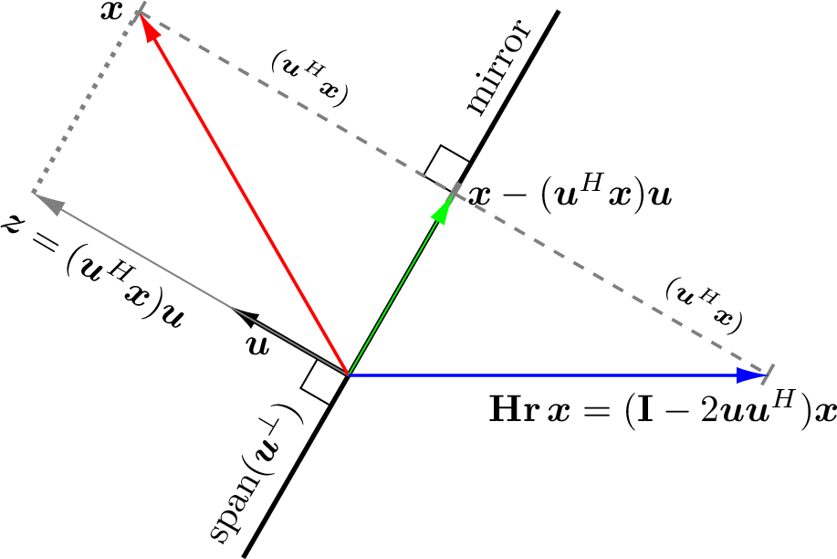
Fig. 12.3 Householder reflector matrix \(\bf{Hr}\) times \(\bm{x}\) is a reflection of \(\bm{x}\) about the hyperplane \(\text{span}(\bm{u}^{\perp})\). We can think of the hyperplane as a mirror. The diagram shows a side view of the mirror. If the vector \(\bm{x}\) is viewed in the mirror, its reflection is the vector \(\mathbf{Hr}\,\bm{x}\). The hyperplane represents the vector space perpendicular to the \(\bm{u}\) vector.

function H = householder(x, n, k)
% HOUSEHOLDER - Find Householder reflection matrix
%
%  x - Real or complex column vector
%  n - Size of Householder transformation matrix
%  k - Size of the leading identity matrix, probably k-1 if k is
%      the column you are currently working on.
%      H = [eye(k) zeros(k, n-k); zeros(n-k, k) Hr], where Hr is
%      the reflector. Size of Hr is (n-k)-by-(n-k).
%  H - Square n-by-n, Hermitian, unitary reflection matrix.
%  Note: If H is real, then it is not only unitary, but because it
%        is symmetric, it is self-inverted (H == H', H*H == I).
%        This is not true if H is complex (H*H' == I).
%
% see also: BIDIAG, HESSFORM, QRFACTOR, EIGQR, GIVENS

    % Modify the sign function so that sign(0) = 1.
    sig = @(u) sign(u) + (u==0);
    m = size(x, 1);
    % catch trivial cases
    if m < 2 || abs(norm(x(2:m))) < 1e-16
        H = eye(n);
        return;
    end
    if isreal(x(1))     % real case
        x(1) = x(1) + sig(x(1))*norm(x);
        u = x/norm(x);
        Hr = eye(m) - 2*(u*u'); % reflection
    else                % complex case
        expTheta = x(1)/norm(x(1));   % e^{i theta}
        expNegTheta = conj(expTheta); % e^{-i theta}
        x(1) = x(1) + expTheta*norm(x);
        u = x/norm(x);
        Hr = expNegTheta * (eye(m) - 2*(u*u'));
    end
    H = zeros(n);
    H(1:k,1:k) = eye(k);
    H(k+1:n, k+1:n) = Hr;
end    % end of function

In some applications, one might start with \(\bm{x}\) and either the hyperplane or \(\bm{u}\) and then determine the reflection \(\mathbf{Hr}\,\bm{x}\). For our application, we start with \(\bm{x}\), but we need to find the \(\bm{u}\) vector such that all elements of \(\mathbf{Hr}\,\bm{x}\), except for the first, are equal to zero. That is to say that the reflection vector needs to lie on the \(x\) axis. [3]

\[\mathbf{Hr}\,\bm{x} = \begin{bmatrix} c & 0 & \ldots & 0 \end{bmatrix}^T = c\,\bm{e}_1, \; \text{where}\: \bm{e}_1 = \begin{bmatrix} 1 & 0 & \ldots & 0 \end{bmatrix}^T\]

From the geometry and since \(\norm{\bm{x}}_2 = \norm{\mathbf{Hr}\,\bm{x}}_2 = \abs{c}\), \(\bm{u}\) must be parallel to \(\bm{\tilde{u}} = \bm{x} \pm \norm{\bm{x}}_2 \bm{e}_1\). So we can find \(\bm{u}\) simply from \(\bm{x}\) with \(\norm{\bm{x}}_2\) added to \(x_1\) with the same sign as \(x_1\) and then making \(\bm{u}\) a unit vector.

\[\bm{\tilde{u}} = \begin{bmatrix} {x_1 + \text{sign}(x_1)\,\norm{x}_2}{x_2} {\vdots} {x_n} \end{bmatrix}, \qquad \bm{u} = \frac{\bm{\tilde{u}}}{\norm{\bm{\tilde{u}}}_2}\]

The Complex Case

If the first value of \(\bm{x}\) is complex, then an adjustment to the algorithm is needed [GOLUB13]. The objective is to put the complex component into the transformation, such that after the transform is applied, the new vector holds only real numbers. In the equation to find the vector \(\bm{u}\), the sign of the first value of \(\bm{x}\) (\(x_1\)) is replaced with the orientation of \(x_1\) in the complex plane (\(e^{i\theta}\)), which from Euler’s complex exponential equation is just \(x_1\) converted to a unit length complex number \(e^{i\theta} = \cos \theta + i \sin \theta\). [4] Then, to make the first element of the vector a real number when the transform is applied, we multiply the transform by the complex conjugate of \(x_1\), which is \(e^{-i\theta}\). See Euler’s Complex Exponential Equation if you are unfamiliar with complex exponentials.

Each Householder reflection matrix combines an identity matrix, zeros, and a Householder reflector. It sets the reflector in the needed location to affect the desired \(\bf{A}\) column. It uses an identity matrix to leave the previously completed work alone.

\[\begin{split}\mathbf{H}_1 = \mathbf{Hr}_1, \qquad \mathbf{H}_2 = \left[ \begin{array}{c|c} 1 & {\mathbf{0}} \\ \hline {\mathbf{0}} & {\mathbf{Hr}_2} \end{array} \right], \qquad \mathbf{H}_3 = \left[ \begin{array}{c|c} \begin{matrix} 1 & 0 \\ 0 & 1 \end{matrix} & {\mathbf{0}} \\ \hline {\mathbf{0}} & {\mathbf{Hr}_3} \end{array} \right]\end{split}\]

We can verify the unitary property of the Householder reflector matrices with the required relationship \(\mathbf{Hr\,Hr}^H = \mathbf{I}\). Note again that \(\bm{u}^H\bm{u} = 1\), but \(\bm{u}\,\bm{u}^H\) is a matrix. Also, \(\left(\bm{u\, u}^H\right)^H = \left(\bm{u}^H\right)^H\bm{u}^H = \bm{u\, u}^H\).

\[\begin{split}\begin{aligned} \mathbf{I} &= \left(\mathbf{I} - 2\,\bm{u\,u}^H\right)\, \left(\mathbf{I} - 2\,\bm{u\, u}^H\right)^H \\ &=\left(\mathbf{I} - 2\,\bm{u\, u}^H\right)\, \left(\mathbf{I} - 2\,\bm{u\, u}^H\right) \\ &= \mathbf{I} - 2\,\bm{u\,u}^H - 2\,\bm{u\, u}^H + 4\,\bm{u\, u}^H \bm{u\, u}^H \\ &= \mathbf{I} + (-2 - 2 + 4)\,\bm{u\, u}^H \end{aligned}\end{split}\]

12.2.3. Numerical Stability

Orthogonal factoring algorithms are regarded as numerically accurate or stable. We introduced the topic of numerical stability in Numerical Stability and saw that poorly conditioned matrices lead to inaccurate solutions. Recall that a metric for a matrix’s condition is its condition number, \(\kappa(\m{A})\). Poorly conditioned matrices have large condition numbers. Algorithms that require matrix multiplications can increase the matrix’s condition number.

\[\kappa(\m{A\,B}) \leq \kappa(\m{A})\,\kappa(\m{B}), \quad \text{and} \quad \kappa(\m{A}^T\m{A}) = \kappa(\m{A})^2\]

Orthogonal factoring algorithms multiply matrices many times. However, the Householder and Givens transformation matrices are unitary and have a condition number of one. So the condition of the matrix is not degraded by the factoring procedure. We saw in Condition Number that the condition number comes from the matrix’s singular values. The unitary property means that \(\mathbf{U}^T \mathbf{U} = \mathbf{I}\). The singular values are all ones because all of the eigenvalues of an identity matrix are ones.

\[\kappa(\mathbf{A}) = \text{cond}(\mathbf{A}) = \norm{\mathbf{A}}_2 \norm{\mathbf{A}^{-1}}_2 = \frac{\sigma_{max}}{\sigma_{min}}\]

Footnotes:

[1]

We use the more general term unitary rather than orthogonal to include the complex cases. However, the transformation matrices only hold complex elements when their inputs are complex.

[2]

It is unnecessary to calculate the angle \(\theta\). The two coordinates define the cosine and sine of \(\theta\).

[3]

The notation \(\bm{e}_i\) indicates a vector of all zeros except for a one in the \(i{\text{th}}\) position.

[4]

It is not necessary to compute \(\theta\), just express \(x_1\) as a unit-length complex number by dividing by its length.