12.1. Introduction
John G.F. Francis (1934–present) is a brilliant mathematician and computer
programmer. His work between 1959 and 1961 at the National Research Development
Corporation (NRDC) in London changed the world. He found two related algorithms
that solved the eigenvalue problem ( ). Several renowned mathematicians dating back to the first
half of the eighteenth century attempted to solve the eigenvalue problem [1].
He was not an academic researcher as one might expect. He was a professional
computer programmer. He was assisting the British Ministry of Aircraft
Production with stability analysis of airplane designs. He was given matrices
of size
). Several renowned mathematicians dating back to the first
half of the eighteenth century attempted to solve the eigenvalue problem [1].
He was not an academic researcher as one might expect. He was a professional
computer programmer. He was assisting the British Ministry of Aircraft
Production with stability analysis of airplane designs. He was given matrices
of size  representing models of aircraft flutter for which
he needed to find the eigenvalues and
eigenvectors [GOLUB09]. So, he read the literature
that he could find on how others had attempted to solve the eigenvalue
problem. He met Jim Wilkinson, a linear algebra expert from Cambridge
University. He decided to try a strategy that combined the latest
developments from three sources—Wilkinson, Heinz Rutishauser from the
Institute of Applied Mathematics at ETH Zurich, and colleagues Wallace
Givens and Alston Householder from Oak Ridge National Laboratory in
Tennessee. He wrote a program in assembly language that implemented an
algorithm called the QR algorithm. Later, he modified his first
algorithm, creating what he called the QR algorithm with implicit
shifts [2]. Both algorithms, especially the second, worked well.
With encouragement from his boss, Christopher Strachey, he published two
papers [FRANCIS61] and [FRANCIS62] about his algorithms.
Then he moved on to other projects, took another job, and was soon no
longer working on numerical analysis problems.
representing models of aircraft flutter for which
he needed to find the eigenvalues and
eigenvectors [GOLUB09]. So, he read the literature
that he could find on how others had attempted to solve the eigenvalue
problem. He met Jim Wilkinson, a linear algebra expert from Cambridge
University. He decided to try a strategy that combined the latest
developments from three sources—Wilkinson, Heinz Rutishauser from the
Institute of Applied Mathematics at ETH Zurich, and colleagues Wallace
Givens and Alston Householder from Oak Ridge National Laboratory in
Tennessee. He wrote a program in assembly language that implemented an
algorithm called the QR algorithm. Later, he modified his first
algorithm, creating what he called the QR algorithm with implicit
shifts [2]. Both algorithms, especially the second, worked well.
With encouragement from his boss, Christopher Strachey, he published two
papers [FRANCIS61] and [FRANCIS62] about his algorithms.
Then he moved on to other projects, took another job, and was soon no
longer working on numerical analysis problems.
Only a few linear algebra and numerical analysis researchers knew of John Francis, so it took some time for the research community to hear about the two QR algorithms. Householder wrote a book in 1964 [HOUSEHOLDER64] that gave the status of research efforts related to the eigenvalue problem; yet, it provides an incomplete picture of the QR algorithm and does not mention the implicit (Francis) algorithm. However, in the following year, Wilkinson published a book devoted to the topic of the eigenvalue problem that gave considerable coverage to both of Francis’s algorithms [WILKINSON65]. The world knew within a few years that the eigenvalue problem was finally solved. The Francis algorithm and its variants [3] are now widely used in numerical analysis software for various applications. An interesting side note is that because Francis did not continue to work on numerical analysis problems, he was unaware for several years that his second algorithm (implicit QR or Francis) became the accepted solution [GOLUB09].
Why was Francis successful when so many esteemed mathematicians before him failed? Some have suggested that being an outsider to numerical analysis research gave him more freedom to try new things as he was not influenced by biases formed from past successes and failures [GOLUB09] and [GUTKNECHT10]. He certainly worked on the problem at the right time. Heinz Rutishauser’s LR algorithm (The LR Algorithm) was close to solving it [GUTKNECHT10]. The primary change that Francis made to the LR algorithm was to follow the advice of Wilkinson and use the unitary transformation matrices of Givens and Householder [GIVENS58], [HOUSEHOLDER58], [WILKINSON59], [FRANCIS61] instead of an elimination-like algorithm. Francis credits Rutishauser in his first publication, stating that his QR algorithm is similar to the LR algorithm except that the transformations are all unitary, which should improve the numerical stability [FRANCIS61]. The switch to unitary transformations also allowed shifts and deflation, as suggested by Wilkinson [WILKINSON59], to be more effective [WILKINSON65]. Indeed, the accumulated knowledge of all of the past efforts made the time right for Francis. Although Francis’s direct input came only from contemporary researchers Wilkinson, Rutishauser, Givens, and Householder, many previous researchers laid the foundation for his success. In particular, Issai Schur significantly contributed to the knowledge needed to solve the eigenvalue problem.
A brief review of the historical linear algebra literature shows that solving the eigenvalue problem was a high priority at the time of Francis’s efforts. The focus on the eigenvalue problem and matrix factorization became more intense starting in the 1950s after general-purpose, programmable computers became available. Large matrix factorization was impractical for manual calculations. Research efforts on the eigenvalue problem provide the background setting for our narrative here because it, and to a lesser degree, the SVD problem, dominated numerical analysis research from about 1950 to 1970 [GOLUB09], [GUTKNECHT10], [WATKINS10]. Although the eigenvalue problem must be part of our discussion, the primary story we seek is the ubiquitous use of unitary transformation matrices in orthogonal factoring algorithms. It was the strategy of using methods for orthogonal factoring that allowed John Francis’s efforts to be successful.
12.1.1. Matrix Factorizations
When solving a linear algebra problem, matrix factoring is usually the
first and most important step. Consider, for example, the available
options for solving a system of linearly independent equations of the
form  . For pedagogical reasons,
beginning students might be instructed to use Gaussian elimination with
an augmented matrix. Computing the inverse of
. For pedagogical reasons,
beginning students might be instructed to use Gaussian elimination with
an augmented matrix. Computing the inverse of  is not a
good option. However, if is square, then LU decomposition
followed by a substitution algorithm works well. A solution found from
the orthogonal QR decomposition of an over-determined matrix has good
numerical stability. If the factoring procedure yields a diagonal or
triangular system, then a substitution algorithm can quickly find a
solution. If a matrix factor is a unitary matrix, then a matrix
transpose finds its inverse.
is not a
good option. However, if is square, then LU decomposition
followed by a substitution algorithm works well. A solution found from
the orthogonal QR decomposition of an over-determined matrix has good
numerical stability. If the factoring procedure yields a diagonal or
triangular system, then a substitution algorithm can quickly find a
solution. If a matrix factor is a unitary matrix, then a matrix
transpose finds its inverse.
When elimination procedures are used to factor a matrix, each step of
the procedure shifts a matrix element to zero, which is offset by
entries in another matrix factor such that the multiplication of the
factors restores the original matrix. For example, in LU decomposition
( ), row operations are applied to to produce
the upper triangular
), row operations are applied to to produce
the upper triangular  . Correspondingly, entries are added
to lower triangular
. Correspondingly, entries are added
to lower triangular  such that multiplying
and together yields a product equal to .
The objective is to produce triangular factors that can be used with
substitution to solve a system of equations (
such that multiplying
and together yields a product equal to .
The objective is to produce triangular factors that can be used with
substitution to solve a system of equations ( ).
).
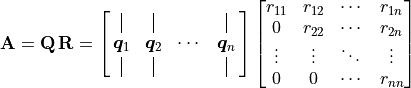
Orthogonal matrix factoring algorithms use a different strategy.
Transformation matrices are designed to change matrix elements to zeros
with multiplication. For example, the QR decomposition
( ) algorithm sequentially uses
Householder transforms,
) algorithm sequentially uses
Householder transforms,  , that when multiplied to
give zeros below the diagonal of the
, that when multiplied to
give zeros below the diagonal of the  column. Matrix
  starts as but moves closer
to upper triangular form with each procedure on the columns
(
starts as but moves closer
to upper triangular form with each procedure on the columns
( ). The product of
transposed transformation matrices forms the
). The product of
transposed transformation matrices forms the  matrix,
 .
.
12.1.2. Factorizations that use the Orthogonal Strategy
The QR decomposition finds factors and ,
where contains orthogonal column vectors, and
is an upper triangular matrix, such that
 . A reliable procedure uses
the QR decomposition to solve square and rectangular systems of
equations. The QR eigendecomposition algorithm also uses the QR
decomposition.
. A reliable procedure uses
the QR decomposition to solve square and rectangular systems of
equations. The QR eigendecomposition algorithm also uses the QR
decomposition.
The eigendecomposition finds the eigenvalues and eigenvectors of a
matrix such that  ,
(
,
(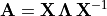 ) where the eigenvectors are the
columns of
) where the eigenvectors are the
columns of  and the eigenvalues,
  , are the
diagonal values of the
, are the
diagonal values of the  matrix.

Each eigenpair,  ,
,  , satisfies the
relationship
, satisfies the
relationship  , which
is to say that multiplying the matrix by one of the
eigenvectors yields a vector equal to the eigenvector scaled by its
eigenvalue. The multiplication does not result in a rotation of the
eigenvector.
, which
is to say that multiplying the matrix by one of the
eigenvectors yields a vector equal to the eigenvector scaled by its
eigenvalue. The multiplication does not result in a rotation of the
eigenvector.
While only the eigendecomposition of a symmetric matrix is orthogonal, the algorithm that finds the eigendecomposition uses two orthogonal factoring algorithms–Hessenberg decomposition and Schur decomposition. The final step of the eigendecomposition of a non-symmetric matrix is multiplying the unitary Schur vectors by the eigenvectors of the upper triangular factor of the Schur decomposition. Thus, the process employs orthogonal factoring methods even though the eigenvector matrix does not usually have orthogonal columns.
The singular value decomposition (SVD) has many data analysis applications and provides solutions to many linear algebra problems (The Singular Value Decomposition, Singular Value Decomposition (SVD) and [MARTIN12]). However, the classic algorithm for calculating the factors suggested that a solution to the eigenvalue problem was a prerequisite, so efforts to find an efficient SVD algorithm were less active until the 1960s. The modern SVD algorithm relies exclusively on unitary transformation matrices and is a variant of the Francis algorithm used to find the Schur decomposition.
Every matrix has an SVD factoring. Square, rectangular, complex, and
even singular matrices have SVD factors. The factoring is
 . Both and
  are orthogonal
matrices. The
are orthogonal
matrices. The  matrix is a diagonal matrix of
positive, real, scalar values that we call the singular values.
matrix is a diagonal matrix of
positive, real, scalar values that we call the singular values.
For a square, full-rank matrix, the factors look as follows.

12.1.3. Definitions
Let us review a few definitions before describing the unitary transforms.
- Transformation Matrix
A transformation matrix, or a transform, changes a vector or another matrix by matrix multiplication. For example, the transformation matrix
 changes matrix
 into
into  as follows.
- Orthonormal Columns
A matrix,
, has orthonormal columns if the columns
are unit vectors (length of 1) and the dot product between the
columns is zero, which is to say that the columns are orthogonal to
each other.
- Unitary Matrix
A matrix
 is
unitary if it has orthonormal columns and is square. The inverse of
a unitary matrix is its conjugate (Hermitian) transpose,
is
unitary if it has orthonormal columns and is square. The inverse of
a unitary matrix is its conjugate (Hermitian) transpose,
 . The product of these matrices with its
transpose is the identity matrix,
. The product of these matrices with its
transpose is the identity matrix,  , and
, and
 .
.
Note
While the notation  means the transpose of a real matrix,
 indicates a Hermitian complex conjugate transpose. The
elements of the transposed matrix hold the conjugates of the complex
numbers, which means that the sign of the imaginary part of the numbers is
changed. MATLAB’s
indicates a Hermitian complex conjugate transpose. The
elements of the transposed matrix hold the conjugates of the complex
numbers, which means that the sign of the imaginary part of the numbers is
changed. MATLAB’s ’ (apostrophe) operator performs a Hermitian
transpose.
- Orthogonal Matrix
A matrix is orthogonal if its elements are real,
 , and it is unitary.
