13.6. All About the Number e
This section is devoted to topics related to the irrational number \(e \approx 2.718281828459046\), which is also called the Euler number. We know from Systems of Linear ODEs that the special number \(e\) is important to solutions to ordinary differential equations (ODEs). When \(e\) is raised to a complex number, the equation represents oscillations, which are important for stability analysis of control systems and converting time and spatial domain data into the frequency domain. The number \(e\) is also used to calculate compound interest rates for savings and loans.
13.6.1. Definition and Derivative
The importance of the number \(e\) to ODEs stems from the derivative of exponential equations of \(e\). If a function is defined as the following, where \(a\) is a real constant and \(x\) is a real variable,
then
Let us now regard exponential equations of \(e\) as special cases of a more general class of exponential equations. In doing so, we will see some interesting properties of \(e\) and also get a start toward finding a definition of the value of \(e\). In the following equation, \(k\) is any positive, real number.
A strategy for finding the derivative of \(y(x)\) is first to take the natural logarithm of \(y(x)\) (base \(e\) logarithm, denoted as \(\ln y\)). Although we have not yet found the value of \(e\), we know that it is a number and can abstractly use it as the base for a logarithm.
The left side of the above equation is more difficult to find. We can use implicit differentiation and the chain rule to find the derivative.
Thus after multiplying by \(y\) we have,
If \(k = 2\), \(\frac{dy}{dx} = a\,(0.693147)\,2^{a\,x}\).
If \(k = e\), \(\frac{dy}{dx} = a\,e^{a\,x}\).
If \(k = 3\), \(\frac{dy}{dx} = a\,(1.0986)\,3^{a\,x}\).
Equation (13.4) is useful, but it assumes that we already know the value of \(e\). We need to use the definition of a derivative to find an equation for the value of \(e\),
We will let \(a = 1\) in the remaining equations.
Relating the last equation to equation (13.4), we find a limit equation for \(\ln{k}\).
Let us test this with the natural log of 2 and 3. We need a very small value for \(h\) to get a reasonably accurate result.
>> h = 0.00000001;
>> ln2 = (2^h - 1)/h
ln2 =
    0.693147184094300
>> log(2)
ans =
    0.693147180559945
>> ln3 = (3^h - 1)/h
ln3 =
    1.098612290029166
>> log(3)
ans =
    1.098612288668110
We can let \(k = e\) and \(\ln{(k = e)} = 1\) to find an equation for the value of \(e\).
To solve for \(e\), we need to change the limit.
Raise both sides to the \(N\) power.
Let us test it with MATLAB. Here, the limited digital resolution of the computer can limit the accuracy if \(N\) is too large.
>> N = 1E10;
>> (1 + 1/N)^N
ans =
    2.718282053234788
>> exp(1)
ans =
    2.718281828459046
The limit can also be used to find powers of \(e\).
13.6.2. Euler’s Complex Exponential Equation
When the exponent of the number \(e\) is a complex number, we see the presence of oscillation.
Here, we follow the engineering practice of using the variable \(j\) for the imaginary number \(\sqrt{-1}\) rather than the math practice of using \(i\).
We can see how \(e^{j\,x}\) relates to the \(\sin(x)\) and \(\cos(x)\) functions by looking at the Maclaurin series for these functions.
The needed Maclaurin series are:
Now replace \(x\) in the equations for \(e^x\) with \(jx\). Remember that \(j^2 = -1\).
Euler’s formula is the relationship between complex exponentials of \(e\) to the cosine and sine functions in the complex plane (\(\mathbb{C}^2\)).
13.6.3. Numerical Verification of Euler’s Formula
If the derivation of Euler’s formula from the Maclaurin series didn’t
convince you, we can try some numerical analysis to show that complex
exponentials produce complex, sinusoidal functions. We will use the
definition of \(e^x\) from equation (13.6). We
expect to see a circle in \(\mathbb{C}^2\), just as we would by
plotting \(\cos \theta + j\,\sin
\theta,\: 0 \leq \theta \leq 2\,\pi\). The plot is shown in figure
Fig. 13.3. We assign \(N\) to be a fairly large
number in the cmplxEuler script . Since
the definition uses a limit as \(N\) goes to infinity, the results
become more accurate when a larger value for \(N\) is used.
% File: cmplxEuler.m
% let n = some big number
N = 100000;
z = linspace(0,2*pi); % test 100 numbers between 0 and 2*pi

% Now show that e^jz = cos(z) + j*sin(z)
% Begin with the definition of the value of e^z.
%    e^z = lim(N = infinity) (1 + z/N)^N
eulerValues = complex(1, z/N).^N;

% This should plot a unit circle, just like
% figure, plot( cos(z), sin(z));
figure, plot(real(eulerValues), imag(eulerValues));
axis equal tight
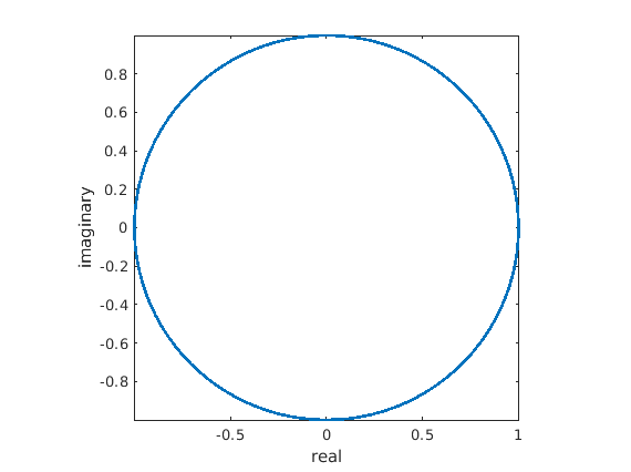
Fig. 13.3 Points along a complex unit circle—numerical verification of Euler’s formula.
13.6.4. Compound Interest
Another application of the number \(e\) relates to one way to calculate interest on loans or savings accounts.
Loans normally use simple interest to track the current principal. The interest paid at each payment is the product of the previous principal, the daily interest rate, and the number of days between payments. The interest is taken from the payment, and the remainder is applied to the principal.
Saving accounts normally use compound interest where the interest is calculated on the principal amount and the accumulated interest of previous periods can thus be regarded as “interest on interest.”
If you invest \(P\) dollars without continued contribution, then the balance of your savings after each compound period (\(t\)) is described by
where \(I\) is the annual interest rate and \(N\) is the number of times the interest is compounded yearly. If interest were compounded continuously, then we would have
If a loan uses compound interest, the principal can grow multiple times between each payment, depending on how often it is compounded. So, the borrower will pay much more. Fortunately, automobile loans and home mortgages use simple interest. However, credit card debt and student loans are more likely to use compound interest.
The difference between simple and compound interest made for a humorous exchange between George Washington, the first president of the United States, and his stepson. Washington’s wife, Martha, was previously the widow of a wealthy man. One of Martha’s sons, John Parke Custis, was not very knowledgeable about business matters when he borrowed money at compound interest to purchase a plantation. When Washington learned of the terms of the loan, he wrote the following to his stepson, “No Virginia estate (except a few under the best management) can stand simple interest. How then can they bear compound Interest?” [NtlArchive].
Footnote:
