5.4.1. The Unicycle Model
Dealing with the displacement and velocities of the two wheels of a
differential drive robot is messy. A preferred model is that of a unicycle,
where we can think of the robot as having one wheel that can move with a
desired velocity ( ) at a specified heading (
 ). Having
the equations to translate between the unicycle model and our wheel
velocities is what allows us to simplify the robot with the unicycle model.
We have seen how to take measured wheel displacements to calculate the new
robot pose. Now we do the reverse and calculate the desired wheel
velocities from the unicycle model. Note the temporary assumption of holonomic
robot movement, which we will soon correct for differential drive robots.
). Having
the equations to translate between the unicycle model and our wheel
velocities is what allows us to simplify the robot with the unicycle model.
We have seen how to take measured wheel displacements to calculate the new
robot pose. Now we do the reverse and calculate the desired wheel
velocities from the unicycle model. Note the temporary assumption of holonomic
robot movement, which we will soon correct for differential drive robots.
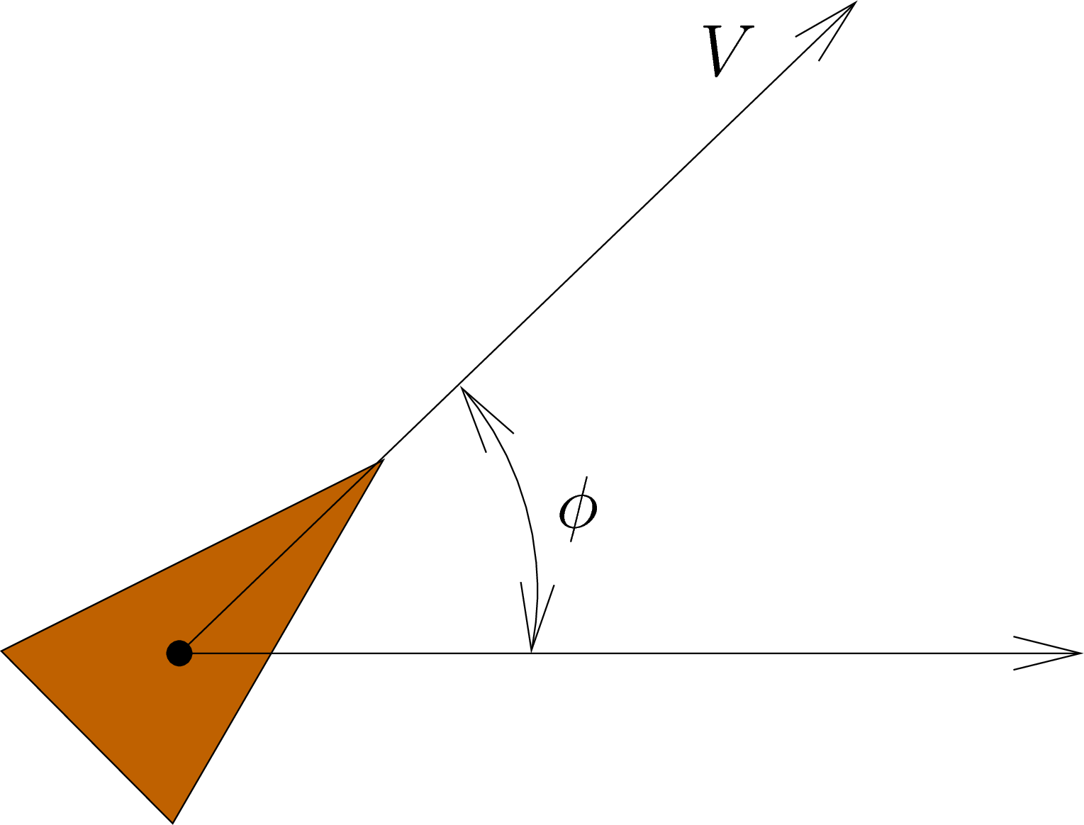
Fig. 5.4 The Simplified Unicycle Robot Model
Note
We represent the measured forward velocity and robot orientation
with variables  and
and  . The desired speed
and direction are represented with the unicycle model using variables
and .
. The desired speed
and direction are represented with the unicycle model using variables
and .
In the global coordinate frame, we can represent the velocity of the unicycle robot as:
(5.1)¶![\mathcal{U} = \left[ \begin{array}{c}
\dot{x} \\ \dot{y} \\ \dot{\phi}
\end{array} \right]
= \left[ \begin{array}{c}
V \!\cos\,\phi \\
V \!\sin\,\phi \\
\omega
\end{array} \right]](../../_images/math/2a8aab1cb278dd55159b4c6afb84a5dde87c1b8f.png)
5.4.1.1. The Jacobian
The kinematics of mechanical systems are often described in terms of
Jacobian matrices. A Jacobian defines how movement of parts of a system
affect the movement of the whole or a larger part of the system. Let
 be the velocity vector of the system,
  be the
pose of the system, and
be the
pose of the system, and  be the pose vector of certain parts of
the system.
be the pose vector of certain parts of
the system.

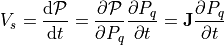
We can calculate the robot velocity relative to the velocities of the left and right wheels. Recall from Updating the Robot Position that the kinematics of directional drive systems gives us the forward and rotational displacement of the robot within a short time interval based on the displacement of the left and right wheels. The forward and rotational velocities can also be computed using the velocity of the left and right wheels. The forward velocity is the average of the wheel velocities.
Note
Remember that  and
and  have units of radians/second,
while has units of meters/second. Multiplying by R, which is
the radius of the wheels (meters/radian) does the unit conversion.
have units of radians/second,
while has units of meters/second. Multiplying by R, which is
the radius of the wheels (meters/radian) does the unit conversion.
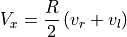
The rotational velocity is the difference of the wheel velocities divided by
the radius of rotation. In robotics literature, the radius
of rotation is  , or the distance between the wheels. One way to
think of this is to consider the case when the left wheel is stopped while
the right wheel moves forward. The robot will rotate about the left wheel
making an arc with radius of .
, or the distance between the wheels. One way to
think of this is to consider the case when the left wheel is stopped while
the right wheel moves forward. The robot will rotate about the left wheel
making an arc with radius of .
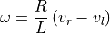
In the local coordinate frame,
the three components of the robot velocity are its
forward velocity (), its perpendicular velocity ( ) and
its rotational velocity (
) and
its rotational velocity ( ) in radians per
second. Differential Drive robots can not move perpendicular to the
direction of wheel rotation, so is always zero. This is the
non-holonomic constraint of a differential drive system.
) in radians per
second. Differential Drive robots can not move perpendicular to the
direction of wheel rotation, so is always zero. This is the
non-holonomic constraint of a differential drive system.
(5.2)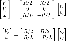
Thus,
In the global coordinate frame, the velocity vector is the time derivative of the pose.
![\dot{\mathcal{P}} = \left[ \begin{array}{c}
\dot{X} \\ \dot{Y} \\ \dot{\theta}
\end{array} \right]
= \spalignmat{\cos \theta, 0; \sin \theta, 0; 0, 1}
\spalignvector{V_x; \omega}](../../_images/math/16999fbfca3c15c1bc38b97ef84358eb7d9e383e.png)
Note
Another gotcha to pay attention to is the units used when expressing velocities.
Since our Optical Encoders do not know the size of wheels on the robot, they report displacement or velocities in terms of radians. Wheel velocities (
and ) are in terms radians per
second. Forward velocities in the Unicycle and Jacobian equations
use linear measurements.Meters or meters per second are the most common linear measurements used.
In equations, the radius of the wheels is usually represented with the letter
 .
.
When we talk about the rotational velocity, we are describing its velocity towards turning, so the unit of radians here is the distance between the directional drive wheels. It is sometimes called the base length and in equations, it usually represented with the letter
.
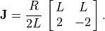
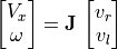
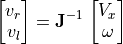
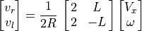
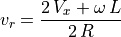
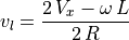
5.4.1.2. Calculating Wheel Velocities
Starting with the desired forward and rotational velocities, we can calculate
the desired wheel velocities. Using the above equations for and
 , we can use either the inverse of the Jacobian or equation
substitution with some simple algebra to come up with the needed equations.
, we can use either the inverse of the Jacobian or equation
substitution with some simple algebra to come up with the needed equations.
A desired forward velocity () is an expected input for steering the
robot towards a goal, but we don’t normally think of a steering heading in
terms of a rotational velocity (). So we need a controller,
either a Proportional Control (P – regulator) or The Point Forward Steering Controller.