2.3. The PID Controller
2.3.1. Proportional Control (P – regulator)
The simplest controllers, which it should be noted are adequate for many situations, produces an output proportional to the error between the observed result and the desired set point. This solutions tends to be slow to reach a steady state response and sometimes oscillates.
Suppose you are in the driver’s seat of your stopped car (in a safe location, of course). You press the accelerator a quarter way down and hold it at that position. The car will start moving and speed up until the drag on the car off-sets the amount of gas sent to engine and it reaches a steady state speed. This scenario, with a constant output to the motor, describes an over-damped controller where the output slowly reaches a steady state position.
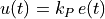
If the output of the controller is proportional to the error between the measured result and set point, then the result will be under-damped such that it will reach the approximate set point quickly, but will often oscillate about the set point before reaching steady state.
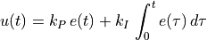
2.3.2. Proportional Integral Control (PI regulator)
To correct the case where the output falls short of the desired output, we can add a term proportional to the area under the time domain error curve. From calculus, we learn that an integral is a way to calculate the area under a curve. Such a term will respond fairly slowly, but in time will contribute just the right amount such that the error between the reference and output goes to zero.
2.3.3. Proportional Integral Derivative Control (PID)
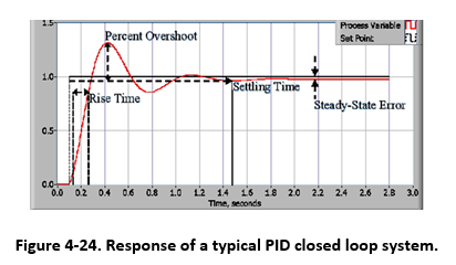
To produce a critically damped result, where it reaches the set point quickly, but has minimal oscillation, we need a derivative term. From calculus, we learn that a derivative measures the rate of change (in our case, with respect to time). If our output is rapidly increasing, then the derivative of the error will be a negative number. If the output is decreasing, then the derivative of the error will be posititve. If the output is changing slowly (near steady state), then the derivative will be a small number. Thus a derivative term will tend to counteract oscillation, but will have minimal impact on the steady state condition.
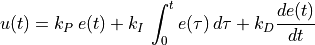
We call our final controller a PID controller.
The biggest challenge with corectly using a PID controller is to
correctly determine the three constants:  ,
,  and
and
 .
.
Here is an Example LabVIEW PID Controller.