5.4.2. The Point Forward Steering Controller
The two other controllers discussed, Linear Time-Invariant Control Theory and The PID Controller, are very powerful, general purpose controllers. Unfortunately, they both require tuning that is difficult to do and is part science, art form and luck. Fortunately, for one of the main problems that we need to solve with mobile robots, there is a clever trick of trigonometry that creates a controller that works fairly well and is not difficult to tune. This controller may be used to provide Go To Angle behavior for a mobile robot using Differential Drive.
The Go To Angle behavior is one of the most basic mobile robot behaviors.
It is a major component the Go To Goal behavior, but is useful for other
objectives also. If the pose of the robot is oriented at  , but
the The Unicycle Model calls for the robot to turn to angle
, but
the The Unicycle Model calls for the robot to turn to angle  , the
Go To Angle controller will move the robot forward while rotating it in
the direction of . The rotation needed is
, the
Go To Angle controller will move the robot forward while rotating it in
the direction of . The rotation needed is
 .
.
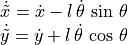
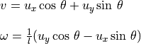
Rather than tracking the robot’s orientation and adjusting the rotational
velocity ( ) with a PID controller, this controller performs a
direct transformation of the unicycle model so that the desired
) with a PID controller, this controller performs a
direct transformation of the unicycle model so that the desired  and can be directly calculated with a simple equation. The
trick of this controller is that it considers a new point on the robot to
calculate the needed Jacobian, and thus the needed wheel velocities. When
we calculate the robot’s pose, we compute the position and orientation of
the center of the robot
and can be directly calculated with a simple equation. The
trick of this controller is that it considers a new point on the robot to
calculate the needed Jacobian, and thus the needed wheel velocities. When
we calculate the robot’s pose, we compute the position and orientation of
the center of the robot  , which is the point half way between the
two drive wheels. Because the robot can not move perpendicular to its
wheels, the second term of The Jacobian is always zero. The robot moves
in the direction of its orientation, , but The Unicycle Model
requires movement in the direction of . This constraint limits
our ability to directly apply The Unicycle Model in our control algorithm. We
would like to take the derivative of with respect to time and set
it equal to the velocity vector
, which is the point half way between the
two drive wheels. Because the robot can not move perpendicular to its
wheels, the second term of The Jacobian is always zero. The robot moves
in the direction of its orientation, , but The Unicycle Model
requires movement in the direction of . This constraint limits
our ability to directly apply The Unicycle Model in our control algorithm. We
would like to take the derivative of with respect to time and set
it equal to the velocity vector  from The Unicycle Model,
but no and can satisfy such an equation.
from The Unicycle Model,
but no and can satisfy such an equation.
![\mathcal{U} = \left[ \begin{array}{c}
u_x \\ u_y \\
\end{array} \right]
= \left[ \begin{array}{l}
V\,\cos \phi \\ V\,\sin \phi
\end{array} \right]
\neq \dot{X}
= \left[ \begin{array}{l}
v\,\cos \theta \\ v\,\sin \theta
\end{array} \right]](../../_images/math/8db0864722c50c51854e6401df570479e1cedc96.png)
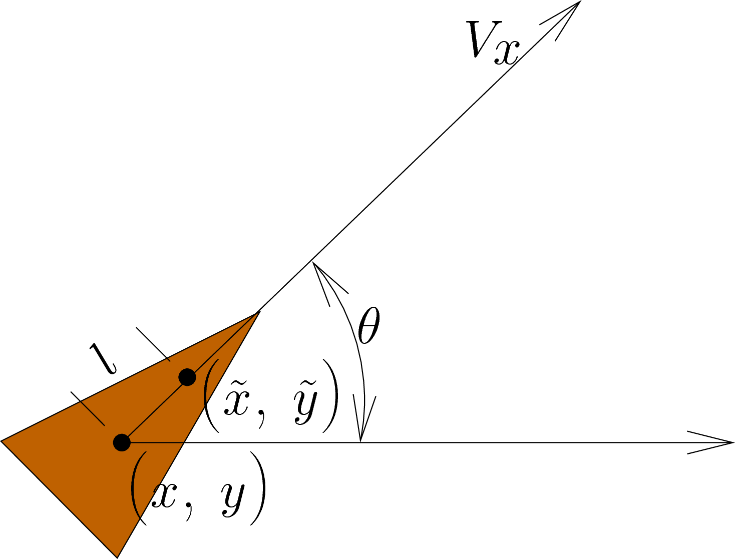
However, such is not the case for a new point  , which is positioned a small distance,
  ,
directly in front of . The point
,
directly in front of . The point  can simultaneously
move forward, perpendicular and rotate. is close to
and once we align the robot with our target destination
(
can simultaneously
move forward, perpendicular and rotate. is close to
and once we align the robot with our target destination
( ) then will pass over the location of
shortly after is at that location.
Thus, as a close approximation to the ideal, we will design a controller
to satisfy
) then will pass over the location of
shortly after is at that location.
Thus, as a close approximation to the ideal, we will design a controller
to satisfy  .
.
For now, do not worry about the value of . After we complete the
analysis, reasonable ranges for will be obvious and computer
simulations, can help us tune . Note that this controller has only
one variable to tune, which makes it easier to use than other controllers.
Warning
Beware of Angles
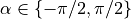
Angles can be tricky because they are linear between  and
and
 , yet they are circular in that and are
in fact the same angle. Another issue with angles is that the atan
function (arctangent) requires division
, yet they are circular in that and are
in fact the same angle. Another issue with angles is that the atan
function (arctangent) requires division  , which is not defined
when
, which is not defined
when  . The solution is this is to use atan2 to compute
angles and to wrap any linear angle calculations to the range
. The solution is this is to use atan2 to compute
angles and to wrap any linear angle calculations to the range
 .
.
To prevent a division by zero, atan2 takes two parameters: alpha = atan2(dy, dx)
Angle wrapping may be performed in either of two methods in traditional programming languages. This is what it would look like in Python:
alpha = math.atan2(math.sin(alpha), math.cos(alpha))

alpha = ((math.pi + alpha) % 2*math.pi) - math.pi
In MATLAB:
alpha = wrapToPi( alpha );
Note
Two things to never do in robot code with angles
Use angles in degrees. All of the math functions return and expect angles in radians. As a general rule, only use degrees to accept and display angle measurements in the user interface. If degrees are used in the user interface, the user interface portion of the code should convert the angles to or from radians so that the robot code always works with angles in radians.
Use the range of an angle as
 . The range
of angles should always be .
. The range
of angles should always be .
5.4.2.1. Controller Derivation
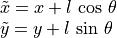
Let us use to define the location of . Then we can
take the derivative of and set it equal to the desired
velocity vector  from the unicycle model. We will use rectangular
coordinates for the initial calculations.
from the unicycle model. We will use rectangular
coordinates for the initial calculations.
Note
Derivatives of trigonometry functions where the angle is a function of time:
From Using Odometry to Track Robot Movement, we know that:

By substitution:
Note
Don’t confuse the names of the velocity variables.  is the
forward velocity calculated from our odometry measurements.
is the
forward velocity calculated from our odometry measurements.  is a
constant value from the unicycle model. If the robot is driving straight,
it is the robot’s velocity. With other controllers used to set the
orientation angle, the forward velocity is not changed. With this
controller, the forward velocity changes with time, so we call it
to indicate that it is a function of time (
is a
constant value from the unicycle model. If the robot is driving straight,
it is the robot’s velocity. With other controllers used to set the
orientation angle, the forward velocity is not changed. With this
controller, the forward velocity changes with time, so we call it
to indicate that it is a function of time ( ).
).
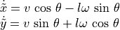
Now, we equate to  to the desired velocity vector.
We will also separate and into a matrix of it’s own
since they are the variables that we want to solve for.
to the desired velocity vector.
We will also separate and into a matrix of it’s own
since they are the variables that we want to solve for.
(5.3)¶![\begin{array}{ll} \mathcal{U} & = \left[ \begin{array}{c}
u_x \\ u_y \\
\end{array} \right]
= \left[ \begin{array}{l}
V\,\cos \phi \\ V\,\sin \phi
\end{array} \right] \\ \\
& = \dot{\tilde{X}}
= \underbrace{\left[ \begin{array}{rl}
\cos\,\theta & -\sin\,\theta \\
\sin\,\theta & \cos\,\theta
\end{array} \right] }_{R(\theta)}
\left[ \begin{array}{cc}
1 & 0 \\
0 & l
\end{array} \right]
\left[ \begin{array}{c}
v \\
\omega
\end{array} \right]
\end{array}](../../_images/math/5d4112c819973bbff457e9f7ef2897e2cc21397b.png)
To solve for and , we need to take the inverse of two
of the above matrices to isolate ![[ v, \omega]](../../_images/math/1ba09798d99e8f9f10d85c6cb73e926472bea7a3.png) on one side of the
equality.
on one side of the
equality.
The matrix identified as  is a known matrix with
some special properties. It is called the rotation matrix. To rotate any
point
is a known matrix with
some special properties. It is called the rotation matrix. To rotate any
point ![[x, y]](../../_images/math/ab8e41dbecb4cdfe7c77ca4911133390a53be3c9.png) by radians counter clockwise, simply
multiply the point by . The inverse of
has a nice property,
by radians counter clockwise, simply
multiply the point by . The inverse of
has a nice property, 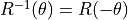 . If multiplying
rotates a point counter clockwise, then multiplying by
. If multiplying
rotates a point counter clockwise, then multiplying by
 will do the inverse and rotate a point the same amount
clockwise.
will do the inverse and rotate a point the same amount
clockwise.
See also
Here is an easy to follow explanation of how to compute the inverse of a matrix: http://www.mathsisfun.com/algebra/matrix-inverse.html
![\left[ \begin{array}{c}
v \\ \omega \\
\end{array} \right]
= \left[ \begin{array}{rr}
\cos\,-\theta & -\sin\,-\theta \\
\sin\,-\theta & \cos\,-\theta
\end{array} \right]
\left[ \begin{array}{cc}
1 & 0 \\
0 & 1/l
\end{array} \right]
\left[ \begin{array}{c}
u_x \\
u_y
\end{array} \right]](../../_images/math/562274f0c47864bc2e99b8a20f699fbaa38230cc.png)
Note
Here are some trigonometry identities that the following equations will use:
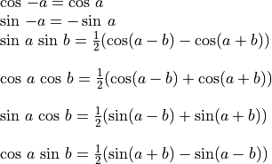
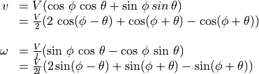
By multiplying the above matrices and applying trigonometry identities, we get:
Replacing  and
and  with their values from the unicycle
model gives us equations in terms of , ,
and .
The trigonometry identities allow us to simplify the equations.
with their values from the unicycle
model gives us equations in terms of , ,
and .
The trigonometry identities allow us to simplify the equations.
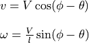
The variables of the final control parameters resolve to  ,
which is the error between current orientation and the desired orientation
angle. For convenience, we can call the error angle,
,
which is the error between current orientation and the desired orientation
angle. For convenience, we can call the error angle,  . As always, when dealing with angles, take care to wrap
 to between and .
5.4.2.2. Observations on the Controller
It is curious that this controller makes changes to as well as to
. The PID controller for Go To Angle behavior only adjusts
. When or is zero is some concern to us.
When
 ,
,  and
and
 or
or  . At
. At  , the robot is at the
desired angle and it is driving forward as desired. At
, the robot is at the
desired angle and it is driving forward as desired. At  ,
the robot is driving in reverse. In some cases, it may be desired to drive
in reverse to a goal. If it drove very long in reverse, it would likely
eventually get off its reverse course and turn around. Depending on the
application, it may be desired to force a turn around by putting tighter
limits on the range of , perhaps between
,
the robot is driving in reverse. In some cases, it may be desired to drive
in reverse to a goal. If it drove very long in reverse, it would likely
eventually get off its reverse course and turn around. Depending on the
application, it may be desired to force a turn around by putting tighter
limits on the range of , perhaps between  and
and
 .
.When
 ,
,  and
and
 or
or  . Here, the robot will briefly
pivot in place, causing to quickly change such that the robot
will begin to move forward while continuing to rotate.
. Here, the robot will briefly
pivot in place, causing to quickly change such that the robot
will begin to move forward while continuing to rotate.
5.4.2.3. Wheel Velocities
From Calculating Wheel Velocities, we know how to calculate the velocities from
and :
Substituting equation (5.4), we get:
Note
has units of meters per second.  and
and  are
in radians per second.
are
in radians per second.
Note
In our programs it may be desired for wheel velocities to be a linear velocity, such as meters / second. So we may want to account for the wheel radius (
 ) in lower portions of
the code, so that the term may be removed from the
equations.
) in lower portions of
the code, so that the term may be removed from the
equations.The term
 can be regarded as a single tunable
parameter,
can be regarded as a single tunable
parameter,  , which acts as a turning gain constant in our
programs.
, which acts as a turning gain constant in our
programs.  seem reasonable.
In the global coordinate frame,
 . In the
local coordinate frame, is the desired heading.
. In the
local coordinate frame, is the desired heading.In our programs, our wheel velocity equations for the Go To Angle controller become:


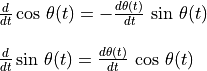
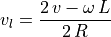
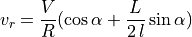
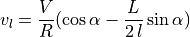
The following graph shows the wheel velocities for  and
and
 . The only variable to tune is (or , if
you prefer). Changes to only changes the maximum velocity for
each wheel and the exact angle for which a wheel might cross stop and change
directions. The basic properties of the plots do not change.
. The only variable to tune is (or , if
you prefer). Changes to only changes the maximum velocity for
each wheel and the exact angle for which a wheel might cross stop and change
directions. The basic properties of the plots do not change.
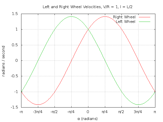
From the graph of the wheel velocities, a few observations can be made.
Except at the exact values of
 , the robot
is always turning towards the desired angle.
(
, the robot
is always turning towards the desired angle.
( and
and  ).
). when
when 
 when
when 
The robot rotates around a stationary wheel at

The robot pivots,
 , at
, at