2.2. Linear Time-Invariant Control Theory
A system is linear when the output is a sum of products between variables and constant coefficients. It is time invariant when the same inputs always yield the same output.
Note
Skimming the surface here
LTI control theory gives us a model to analyize the behavior of a control system. It is used in the study of systems with complex moving parts such as robots used in manufacturing that have arms with several joints and degrees of freedom. Our coverage here is just an introduction.
We can model a controller as being linear and time–invariant (LTI). Controllers that are not linear can often be modeled as being linear within a limited operating range. Analog LTI systems are modeled with differential equations. On computer controlled discrete sampled systems, derivatives become differences in sample values and differential equations become difference equations. The design process for discrete LTI systems uses difference equations and math tools from the field of linear algebra.
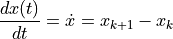
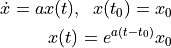
The change to a system from the system plant can be modeled as a function of the current state and control signal.

Then, given a sample time of  .
.
The task of designing the controller then becomes a matter of designing the
control signal ( ) from the error between the reference and
estimated system state.
) from the error between the reference and
estimated system state.
2.2.1. State Space Form
LTI controllers are represented with equations in a standardized format called State Space Form. The first step when designing a controller is to describe the desired behavior in state space form. State space form requires three matrices. Some more complex controllers have a forth matrix also. These matrices will then be used in a standardized design to implement the controller.
A key concept is to focus on modeling the state of the system. The state,
 , is usually a vector containing the physical position of the
system (robot) and the derivative with respect to time for each dimension of
the controller’s position. For simple mobile robots, the state of the robot
is described in two dimensions,
, is usually a vector containing the physical position of the
system (robot) and the derivative with respect to time for each dimension of
the controller’s position. For simple mobile robots, the state of the robot
is described in two dimensions, ![x = \left[ p_x, p_y, \dot{p}_x,
\dot{p}_y \right]](../_images/math/e0331df1b10ad8d3c7c2f4f6b6d676f7d8e7d3b2.png) . Although some robotic controllers, such as speed
control and steering angle, have a single dimension state. Controllers for
arm robots may require a state vector with three dimensions each for the
position and orientation of the end effector.
. Although some robotic controllers, such as speed
control and steering angle, have a single dimension state. Controllers for
arm robots may require a state vector with three dimensions each for the
position and orientation of the end effector.
2.2.2. The Point Mass Controller
To illustrate how to model a controller with state space equations, we will consider the simplest of controllers. In the point mass controller, a force is applied to a point on a line. From physics, we know that a force produces an acceleration (F = ma).

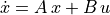
The state of the system is a 1 x 2 vector.
![x = \left[ \begin{array}{c}
x_1 \\ x_2
\end{array} \right]](../_images/math/5e57e7e21f1215ac3061bfe8dd34ca78edcb8078.png)
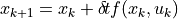
The state space model consists of two equations – the derivative of the state
and the output, which is the controlled position.


To put the above equations in state space form, we express them with a standardized notation as two equations of matrices.
![\dot{x} = \left[ \begin{array}{c}
\dot{x}_1 \\ \dot{x}_2
\end{array} \right]
= \left[ \begin{array}{cc}
0 & 1 \\
0 & 0
\end{array} \right]
\left[ \begin{array}{c}
x_1 \\ x_2
\end{array} \right]
+ \left[ \begin{array}{c}
0 \\ 1
\end{array} \right]
u](../_images/math/35a4cf6f88a4d66b245e283221c0675f34b22add.png)
![y = \left[ \begin{array}{ll} 1 & 0 \end{array} \right]x](../_images/math/82ad25d8d3d382026f5de93f900f7b22f1feaa08.png)
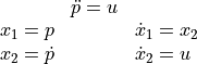
The state space form is:

For the point mass controller,
![A = \left[ \begin{array}{cc}
0 & 1 \\
0 & 0
\end{array} \right]
B = \left[ \begin{array}{c}
0 \\ 1
\end{array} \right]
C = \left[ \begin{array}{ll} 1 & 0 \end{array} \right]](../_images/math/cef189fd5e8d02fad8112619012f6197d545f7f4.png)
2.2.3. The Controller Implementation
We start with the model of the system in state space form:
The matrices  ,
,  and
and  are called the characteristic
matrices. The matrix is called the Dynamics Matrix because it
describes the physics of the system. The matrix is called the
Control Matrix because it operates on the input. The matrix is
called the Sensor Matrix because our estimate of the system position comes
from the sensors. The sensors operate on the internal state of the system to
quantify its current position.
are called the characteristic
matrices. The matrix is called the Dynamics Matrix because it
describes the physics of the system. The matrix is called the
Control Matrix because it operates on the input. The matrix is
called the Sensor Matrix because our estimate of the system position comes
from the sensors. The sensors operate on the internal state of the system to
quantify its current position.

To design a controller, always begin by writing the equations for
 and
and  in the generalized state space form. These
equations describe our model for the controller, not its solution that could be
used to implement the controller. However, there is a known solution for a
controller described by the state space equations.
in the generalized state space form. These
equations describe our model for the controller, not its solution that could be
used to implement the controller. However, there is a known solution for a
controller described by the state space equations.
We will skip the majority of the math to derive the solution. However, we should point out a couple points which relate to the stability of the system.
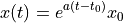
We know from differential equations that if the variables are scalars, instead of matrices, and we ignore the input term that the solution appears as follows.
Note
This simple differential equation solution relates to the determination of if the controller is stable or not.
You may recognize this equation from biology or other related fields. Equations describing growth and decay take this general form.
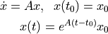
It turns out that we can express the differential equation solution in the same
form when is a matrix.
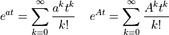
It is a bit awkward to work with equations like this since part of exponent
term is a matrix. However, exponent equations using the special number
 have a Taylor series expansion. By using the Taylor series expansion,
dealing with matrix is simplified.
have a Taylor series expansion. By using the Taylor series expansion,
dealing with matrix is simplified.
The Taylor series expansion relates to the general form of the controller solution.
Note
Controller Equations for LTI discrete systems:
![x[k] = A^k x[0] + \sum_{j=0}^{k-1} A^{k-j-1} Bu[j]](../_images/math/546004672501282002d95d5450f32fa4854afac3.png)
![y[k] = C A^k x[0] + \sum_{j=0}^{k-1} C A^{k-j-1} Bu[j]](../_images/math/480551a396dce24dde14e05ea751ac612e0042e3.png)
This may look difficult and too time consuming to compute for each time sample; however, there are iterative techniques that allow us to reuse previous calculations.
2.2.4. Controller Stability
We discussed previously that the stability of the system is related to
the solution to the differential equation  , which
contains an exponential equation with the special math constant of .
, which
contains an exponential equation with the special math constant of .
The value of the constant  determines if the system is stable or if it
might produce very large values which can not be satisfied by the hardware and
thus, the controller is unstable.
determines if the system is stable or if it
might produce very large values which can not be satisfied by the hardware and
thus, the controller is unstable.

Fig. 2.3 With a positive exponent, the controller blows up – BOOM!

Fig. 2.4 With a negative exponent, the controller is stable
The basic concept is that a negative constant in the exponent equation is
what determines stability or not. Unfortunately, with discrete systems
expressed in state space form, we can not simply evaluate a constant variable.
We can determine stability of the system by evaluating the Dynamic
Matrix, . To do this we need to compute the eigenvalues of the
matrix. The system is stable if the real part of all of the eigenvalues are
negative. It is critically stable if the real part of any eigenvalues are zero.
It is unstable if any eigenvalues have positive real components. If any
eigenvalues have complex components, then the system will oscillate to various
degrees depending on the value of the eigenvalue’s imaginary component.
Note
Eigenvalues come to us from the field of linear algebra. This web page, and the Applied Data Analysis notes talk about how to compute eigenvalues of a matrix. However, it is not necessary to compute them by hand. The eig( ) function in MATLAB and numpy.linalg.eig( ) function in Python will return the eigenvalues of a matrix.
Here is how the eigenvalue computations in Python looks for the point mass system. I’m using iPython in what is shown below.
In [1]: import numpy

In [2]: a = numpy.array([[0, 1],[0,0]])

In [3]: a
Out[3]:
array([[0, 1],
    [0, 0]])

In [4]: numpy.linalg.eig(a)
Out[4]:
(array([ 0.,  0.]),
array([[  1.00000000e+000,  -1.00000000e+000],
    [  0.00000000e+000,   2.00416836e-292]]))
We see here that it has two eigenvalues and that the real and imaginary part of both eigenvalues are zero. Thus, the system is only critically stable. The eig( ) function returned two arrays. The first array is the eigenvalues. The second array relates to eigenvectors, which obviously are related to eigenvalues, but we don’t need them here.
2.2.5. Designing for Stability
We have not discussed the input to our system. Since we want to make use of
feedback to produce a stable controller, we could make the input be a
function of , the estimated output as measured by the sensors. In
doing so, we might be able to design the controller to be strictly stable.
Considering the point mass controller, we could design u to always move the point towards the origin (zero).
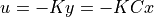
We have a new variable  that we can use to tune the controller.
Since is now in terms of , we can now write the
whole state space model in terms of .
that we can use to tune the controller.
Since is now in terms of , we can now write the
whole state space model in terms of .

Now, if we call 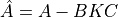 , we have a state space equation that
is just like the differential equation that we looked at before.
, we have a state space equation that
is just like the differential equation that we looked at before.

Thus to determine stability, we can compute the eigenvalues of
 .
.
2.2.5.1. First Try
Let’s set  to start with and see if it is stable.
![\hat{A} = \left[ \begin{array}{cc}
0 & 1 \\
0 & 0
\end{array} \right]
- \left[ \begin{array}{c}
0 \\ 1
\end{array} \right]
\left[ \begin{array}{ll} 1 & 1 \end{array} \right]
\left[ \begin{array}{ll} 1 & 0 \end{array} \right]
= \left[ \begin{array}{cc}
0 & 1 \\
-1 & 0
\end{array} \right]](../_images/math/2009603966ba2aedad4a179d505aba2d894762a4.png)
To determine stability, we can use either Python or MATLAB to find the
eigenvalues of .

Where  is the engineering common name for the imaginary value
 . Math folks mistakenly call it
  , but engineers call
it .
, but engineers call
it .
Thus, with , the system is only critically stable and it
oscillates. We can do better!
2.2.6. Placing Eigenvalues
We can pick the eigenvalues of the system and work backwards to find the desired coefficients.
We’ll begin by combining our previous and terms into one
matrix so that we only need to compute one matrix.
The state space equations are now:
![u = -K\,x =
-\left[ \begin{array}{ll} k_1 & k_2 \end{array} \right]\,x](../_images/math/199718ca0505ccd64881fbd3f0dd495d83f8f738.png)
For the point mass controller,
![\hat{A} = A - BK = \left[ \begin{array}{cc}
0 & 1 \\
0 & 0
\end{array} \right]
- \left[ \begin{array}{c}
0 \\ 1
\end{array} \right]
\left[ \begin{array}{ll} k_1 & k_2 \end{array} \right]
= \left[ \begin{array}{cc}
0 & 1 \\
-k_1 & -k_2
\end{array} \right]](../_images/math/296e700e6b4e0d75b4ad4a6bede1841e17d22fb1.png)
Now, we need to compute the eigenvalues of , but the matrix
contains variables, so we can not use our software tools. MATLAB contains a
function called place that can place the eigenvalues and compute the needed
coefficients. If we forgot to pay MATLAB’s big price tag, then we’ll have to
compute them by hand. But since this is a fairly small matrix, it will not be
so bad.
2.2.6.1. Computing Eigenvalues
Given a matrix M, it’s eigenvalues ( ) satisfy the equation:
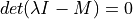
Where  is the identity matrix.
![M = \left[ \begin{array}{cc}
m_1 & m_2 \\
m_3 & m_4
\end{array} \right]](../_images/math/a8b59d14bf1f61a7d5a30b91e8f93807ebf1b6b0.png)
![\lambda \mathit{I} - M = \lambda
\left[ \begin{array}{cc}
1 & 0 \\
0 & 1
\end{array} \right] - M
= \left[ \begin{array}{cc}
\lambda - m_1 & -m_2 \\
-m_3 & \lambda - m_4
\end{array} \right]](../_images/math/a7649774e7708b53eb93e88d076736480765cbca.png)
For a  matrix, the determinant is a scalar given by:
![det\left( \left[ \begin{array}{cc}
a & b \\
c & d
\end{array} \right] \right)
= ad - cb](../_images/math/5ee67c70b750ff2ed92a9d0f4ecff03336e1210c.png)
See the notes for the Applied Data Analysis and Tools course for much more on computing eigenvalues and eigenvectors. (Application of Eigenvalues and Eigenvetors)
2.2.6.2. Back to the Point Mass

We want both eigenvalues to have negative real numbers so that the controller
is stable and does not oscillate. We could set both eigenvalues to  .
Eigenvalues are also called poles, which is a term deriving from evaluation of
analog systems in the LaPlace domain. The point being that if our
variables are at any eigenvalue, a term in a product of poles
becomes zero resulting in the whole product being zero.
.
Eigenvalues are also called poles, which is a term deriving from evaluation of
analog systems in the LaPlace domain. The point being that if our
variables are at any eigenvalue, a term in a product of poles
becomes zero resulting in the whole product being zero.
We represent each eigenvalue as  and write the following
product of poles:
and write the following
product of poles:
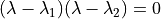
Since we want the eigenvalues at :
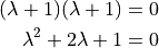
In computing the eigenvalues of the point mass controller, we had:

We can line up the coefficients of the two polynomials to find our
matrix.
![K = \left[ \begin{array}{ll} k_1 & k_2 \end{array} \right]
= \left[ \begin{array}{ll} 1 & 2 \end{array} \right]](../_images/math/d425d7b6d2979742935e4add6b359d25913f43a6.png)
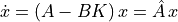
Our state space equations become:
![\dot{x} = (A - BK)\,x = \left( \left[ \begin{array}{cc}
0 & 1 \\
0 & 0
\end{array} \right]
- \left[ \begin{array}{c}
0 \\ 1
\end{array} \right]
\left[ \begin{array}{ll} 1 & 2 \end{array} \right]
\right)\,x
= \left[ \begin{array}{cc}
0 & 1 \\
-1 & -2
\end{array} \right]x](../_images/math/927850500265c68ea2acddea0cf555d80348dd74.png)
![u = -Kx =
\left[ \begin{array}{ll} -1 & -2 \end{array} \right]x](../_images/math/fa2c747382e87af7633183cc0f7b39386156d132.png)
Now, our equation for becomes:
![\hat{A} =
\left[ \begin{array}{cc}
0 & 1 \\
-1 & -2
\end{array} \right]](../_images/math/3d8693cae641bf3921569c56116b1fe520cdd105.png)
Now, we can use use Python to compute the eigenvalues of
.
In [1]: import numpy

In [2]: Ahat = numpy.array([[0, 1],[-1, -2]])

In [3]: numpy.linalg.eig(Ahat)[0]
Out[3]: array([-1., -1.])
Thus, we have verified that both eigenvalues are at . Our controller
is stable and it does not oscillate.
It may seem like we covered a lot in this section, but we really just introduced LTI controllers. We’ll leave more complete coverage to more advanced courses dealing specifically with control systems.