10. Principal Component Analysis (PCA)¶

As the name implies, Principal Component Analysis (PCA) accentuates the principal components of data such that the subtle but salient features of data are more apparent. Like the SVD, PCA reduces the dimensionality of data emphasizing the distinguishing characteristics while removing the uncorrelated noise. The PCA algorithm maps the data into new axes called the PCA space. From the PCA space, the data may be reconstructed with reduced dimension as the rank- $k$ sum of SVD outer products accomplishes. However, it is more common to use the PCA space data for classification applications. In the PCA space, similar items are grouped together and separated from clusters of dissimilar items.

Suppose that you wish to automate the classification of items into groups based on measurable features. PCA can use correlations between the features to find a linear combination of the features such that similar items are clustered together in the reduced dimension PCA space. PCA uses the most significant eigenvectors found from a covariance matrix to find the linear combinations of the features. Then, when we multiply sample data by the most significant eigenvectors (determined by the eigenvalues), the differences between data sets become more obvious allowing for source identification.

If you have $n$ measured features from $m$ sources (samples) then the data can be arranged in a matrix. Examples of potential data sets include the stock values from $m$ companies taken over $n$ days, opinions of $m$ customers regarding $n$ competing products, or the grades of $m$ students in $n$ courses. In the examples presented here, the matrix columns hold the measured features and each row holds the data taken from one source. Although with adjustments to equations, the data may be transposed with the features in rows and the samples in columns.

Use of a covariance matrix is significant to PCA as it reveals how similar and dissimilar (at variance) sets of data are to each other. (See Covariance and Correlation)

The first step in the algorithm is to subtract the mean of each feature from the data so that each feature has a zero mean. This is needed to make a covariance matrix.

$\mathbf{D} = \mat{\vertbar{}, \vertbar{}, {}, \vertbar{}; (\bm{x}_1-\mu_1){}, (\bm{x}_2-\mu_2){}, \cdots{}, (\bm{x}_n-\mu_n){}; \vertbar{}, \vertbar{}, {}, \vertbar{}}$

Recall from Covariance and Correlation that a covariance matrix is symmetric with the variance of each feature on the diagonal and the covariance between features in the off-diagonal positions.

$\mathbf{Cov_x} = \frac{\mathbf{D}^T\,\mathbf{D}}{m - 1}$

$\mathbf{Cov_x} = \mat{Var({x_1, x_1}), Cov({x_1, x_2}), \cdots, Cov({x_1, x_n}); Cov({x_2, x_1}), Var({x_2, x_2}), \cdots, Cov({x_2, x_n}); \vdots, \vdots, \ddots, \vdots; Cov({x_n, x_1}), Cov({x_n, x_2}), \cdots, Var({x_n, x_n})}$

Next, the eigenvectors, $\mathbf{V}$ , and eigenvalues of the covariance matrix are found. The eigenvalues are used to sort the eigenvectors. All eigenvalues could be used, but because we wish to achieve dimensionality reduction, only the eigenvectors with the largest eigenvalues are used. The PCA space is the $k$ most significant eigenvectors. The sub-set of the eigenvectors gives us the mapping of the data onto the PCA space.

$\mathbf{W} = \mat{\bm{v}_1, \cdots, \bm{v}_k}$

Note

The computation performed to find the $\bf{V}$ eigenvector matrix from the $\bf{D}$ matrix is the same as finding the $\bf{V}$ sub-matrix of the SVD ([~, ~, V] = svd(D)).

$\bf{W}$ gives us the linear combinations of each data feature to project the data onto the PCA space, which is found by multiplying the $\bf{W}$ matrix by each sample vector.

$\mathbf{Y} = \mathbf{D\,W}.$

For purposes of classification and object recognition, the data in the PCA space ( $\bf{Y}$ ) is used to display or compare the data.

To reconstruct the original data with reduced dimensionality, we just reverse the steps.

$\begin{array}{ll} \mathbf{\tilde{X}} &= \mathbf{D} + \bm{\mu} \\ &= \mathbf{W\,(W}^T\,\mathbf{D}) + \bm{\mu} \\ &= \mathbf{W\,Y} + \bm{\mu} \end{array}$

Transposed Data

If the measured features are held in the rows with the samples in the columns, then adjusted equations are as follows.

$\mathbf{D} = \spalignmat{\horzbar{} {(\bm{x}_1 - \mu_1)} \horzbar{}; \horzbar{} {(\bm{x}_2 - \mu_2)} \horzbar{}; \vdots{} \vdots{} \vdots{}; \horzbar{} {(\bm{x}_n - \mu_n)} \horzbar{}}$

$\mathbf{Cov_x} = \frac{\mathbf{D\,D}^T}{n - 1}.$

$\mathbf{Y} = \mathbf{W}^T\mathbf{D}.$

10.1. PCA for Data Analysis¶

To illustrate what PCA does with a simple plot, the following code shows a PCA example with only two data sets. Noise was added to the data to show how dimensionality reduction separates the essence of the data from the uncorrelated noise. In this example, the data was reconstructed with reduced dimensionality. Notice the lines showing the principal and minor axes. The orientation of the principal axis is aligned with the correlation of the data, while the minor axis is aligned with the uncorrelated noise. Thus, as we also saw in (Dimensionality Reduction) for the SVD, the lower rank data is preferred to the full rank data that contains noise. Fig. 10.1 shows a plot demonstrating that the reconstructed data is aligned with the correlation between the columns of the original data.

Note

The MATLAB Statistics and Machine Learning Toolbox has a PCA function, but the direct calculation is only a few lines of code.
The PCA_demo example uses the repmat MATLAB function that that has been previously used. The repmat function creates a matrix with copies of a scalar, vector, or matrix. In this case, the variable mu is a row vector, so repmat(mu, m, 1) makes a matrix with $m$ rows, each holding one copy of the mu vector. This allows use of element-wise subtraction of the mean from each column.

% File: PCA_demo.m
% PCA - 2D Example
n = 2;
m = 50;
% two columns random but correlated data
X = zeros(m, n);
X(:,1) = 5*randn(m, 1) - 2.5;
X(:,2) = -1 + 1.5 * X(:,1) + 5*randn(m,1);
X = sortrows(X,1);

%% find PCA from eigenvectors of covariance
mu = mean(X);
D = X - repmat(mu, m, 1);
covx = D'*D/(m - 1);      % sources in rows, features in columns
[V, S] = eig_decomp(covx);
% project onto PCA space
W = V(:,1);               % only use dominant eigenvector
Y = D * W;
disp('Eigenvalue ratios to total')
disp(S/trace(S))
% Data reconstruction
Xtilde = Y*W' + repmat(mu, m, 1);
% plots
figure, scatter(X(:,1), X(:,2)), title('PCA Demo');
hold on
plot([0 5*V(1,1)], [0 5*V(2,1)]);  % principal axis
plot([0 5*V(1,2)], [0 5* V(2,2)]); % minor axis
plot(Xtilde(:,1), Xtilde(:,2));    % principal component
legend({'data in', 'principal axis', 'minor axis', ...
    'reconstruction'}, 'Location', 'northwest');
hold off

function [eigvec,eigval]=eig_decomp(C)
    [eigvec,eigval]=eig(C);
    eigval=abs(diag(eigval)');
    [eigval, order]=sort(eigval, 'descend');
    eigval=diag(eigval);
    eigvec=eigvec(:, order);
end

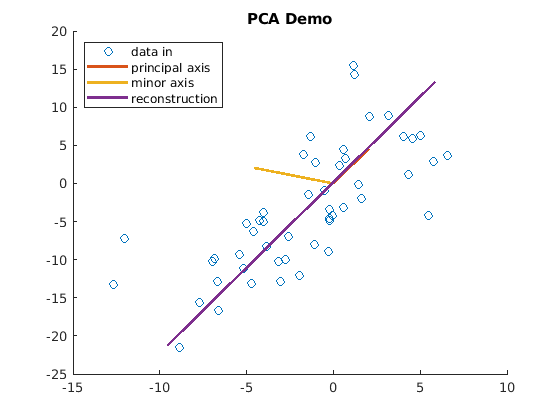
Fig. 10.1 The principal component of the reconstructed data from PCA is aligned with the correlation between the columns of the original data.

Is PCA the same as Least Squares Regression?

The plot in Fig. 10.1 makes it appear that reconstructed data from PCA does the same thing as least squares regression; however, it differs in two ways.

In least squares regression, the error that is minimized is parallel to the $y$ –axis, in PCA the minimized error is orthogonal to the data projection line (principal axis).
In least squares regression, the data fit is an extension of solving a system of linear equations for over-determined systems. In PCA, the data fit is a by-product of dimensionality reduction.

10.2. PCA for Clustering¶

An important application of PCA is classification, which reduces the dimensions of the data for the purpose of making it easier to see how the attributes of items of the same type are similar and differ from items of other types. The result of the analysis is often a plot showing the data in the PCA space. In this example, we will look at a public domain dataset and produce a scatter plot showing how groups of the data are clustered in the PCA space.

The dataset can be downloaded from the Data World web site. It comes from the USDA National Nutrient Database and was made available by Craig Kelly. It list many different foods and identifies food groups, nutrition, and vitamin data for each food. We will use the nutrition information in the PCA analysis. The scatter plot in Fig. 10.2 shows how different food groups are similar. For example, it shows that some fruits and most grains are similar to sweets, probably because they are also high in carbohydrates. Some of the food groups that are contained in the data are not plotted.

To see a list of all food groups in the data set, type the following after the FoodGroups variable is created by the script.

>> categories(FoodGroups)

Download the dataset and my MATLAB script.

nndb_flat.csv

PCA_food.m

Fig. 10.2 Scatter plot of first two principal components from nutrition data for several foods from seven food groups.

10.3. PCA for Recognition¶

A fun example of how PCA can be used is for face recognition. The eigenvectors found from PCA give us a matrix for multiplying images of peoples faces. These resulting matrices, or vectors – depending on the implementation, make a more succinct representation of whom is pictured in each image.

An example implementation is found on the MathWorks File Exchange web site. Two dimensional PCA for face recognition [ALSAQRE19]

Since, like SVD, PCA reduces the dimensionality of the data from rank $r$ to rank $k$ , for purposes of comparing training and testing data, row or column coefficients of the data beyond $k$ may either be removed (making smaller matrices) or set to zero. Reducing the dimensionality is often desired to make the matrix more manageable.

Additional reading

Here is a very good tutorial on PCA Principal_Component_Analysis_Tutorial.pdf by Alaa Tharwat that I found on MathWorks File Exchange ([THARWAT16]). The tutorial shows both the SVD and covariance PCA algorithms. I will use the covariance algorithm. Figure 2 of the tutorial shows a diagram of the covariance algorithm.

Homework

Now complete PCA Data Classification homework.

10. Principal Component Analysis (PCA)¶

10.1. PCA for Data Analysis¶

10.2. PCA for Clustering¶

10.3. PCA for Recognition¶

Table of Contents

Previous topic

Next topic

This Page