4.6. Statistics on Matrices

4.6.1. Column Statistics

When a matrix is passed to a statistical function, the default is to work on each column of the matrix independently. The result is a row vector, which may in turn be used with other statistical functions if desired.

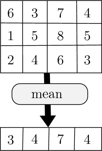
Fig. 4.12 The of a matrix is a row vector containing the means of each column.

Some functions return multiple values for each column. For example, the diff function calculates the difference between adjacent elements in each column of the input matrix. The cumsum function also returns a matrix rather than a row vector.

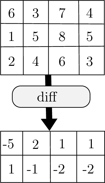
Fig. 4.13 The diff of a matrix is a matrix with one less row holding the differences between the elements of each column.

4.6.2. Changing Dimension

Many statistical functions accept an optional dimension argument that specifies whether the operation should be applied to the columns independently (the default) or to the rows.

If matrix \(\bf{A}\) has size \(10{\times}20\), then mean(A,2) returns a 10 element column vector; whereas, mean(A) returns a 20 element row vector.

Some functions, such as min, max, and diff, use the second argument for other purposes, which makes dimension the third argument. To skip the second argument, use a pair of empty square brackets for an empty vector, [].

>> Amin = min(A,[],2);

4.6.3. Covariance and Correlation

Covariance shows how distinct variables relate to each other. It is calculated in the same manner that variance is calculated for a single variable. Variance (square of the standard deviation) is the expected value of the squared difference between each value and the mean of the random variable. Similarly, the covariance between two variables is the product of the differences between samples and their respective means.

\[\sigma_x^2 = E(X - \mu_x)^2, \quad \sigma_{xy} = E[(X - \mu_x)(Y - \mu_y)]\]

\[s_x^2 = \frac{1}{n - 1} \sum_{i = 1}^n (x_i - \bar{x})^2, \quad S_{xy} = \frac{1}{n - 1} \sum_{i = 1}^n (x_i - \bar{x})(y_i - \bar{y})\]

Thus, the covariance between a variable and itself is its variance, \(s_{xx} = s_x^2\). Covariance is represented with a symmetric matrix because \(s_{xy} = s_{yx}\). The variances of each variable will be on the diagonal of the matrix.

For example, consider taking a sampling of the age, height, and weight of \(n\) children. We could construct a covariance matrix as follows.

\[\begin{split}\mathbf{Covariance}(a, h, w) = \begin{bmatrix} s_{aa} & s_{ah} & s_{aw} \\ s_{ha} & s_{hh} & s_{hw} \\ s_{wa} & s_{wh} & s_{ww} \end{bmatrix}\end{split}\]

The correlation coefficient of two variables is a measure of their linear dependence.

\[r_{xy} = \frac{s_{xy}}{s_x s_y}\]

A matrix of correlation coefficients has ones on the diagonal since variables are directly correlated to themselves. Correlation values near zero indicate that the variables are mostly independent of each other, while correlation values near one or negative one indicate positive or negative correlation relationships. Correlation coefficients are generally more useful than covariance values because they are scaled to always have the same range (\(-1 \leq r \leq 1\)).

\[\begin{split}\mathbf{R}(a, h, w) = \begin{bmatrix} 1 & r_{ah} & r_{aw} \\ r_{ha} & 1 & r_{hw} \\ r_{wa} & r_{wh} & 1 \end{bmatrix}\end{split}\]

The MATLAB functions to compute the covariance and correlation coefficient matrices are cov and corrcoef. In the following example, matrix \(\bf{A}\) has 100 random numbers in each of two columns. Half of the value of the second column comes from the first column, and half comes from another random number generator. The variance of each column is on the diagonal of the covariance matrix. The covariance between the two columns is on the off-diagonal. The off-diagonal of the matrix of correlation coefficients shows that the two columns have a positive correlation.

>> A = 10*randn(100, 1);
>> A(:,2) = 0.5*A(:,1) + 5*randn(100, 1);

>> Acov = cov(A)
Acov =
   94.1505   50.0808
   50.0808   50.6121
>> Acorr = corrcoef(A)
Acorr =
    1.0000    0.7255
    0.7255    1.0000