2.9. Functions Operating on Vectors

2.9.1. Replacing Loops with Vectorized Code

As mentioned in Vectors and Matrices in MATLAB, MATLAB can operate on whole vectors and matrices with a single arithmetic expression. Code that takes advantage of this feature is said to be vectorized. Such code has two benefits over code that uses loops to iterate over the elements of vectors. First and most importantly, writing vectorized code can be simpler and faster than writing code using loops. Secondly, vectorized code runs faster because MATLAB’s interpreter runs less, and optimized, compiled code runs more to perform the calculations.

The functions tic and toc are used in piEstimate to illustrate the difference. More complex expressions yield more speed improvements for vectorized code. The three code sections find the same estimate for \(\pi\), but the vectorized code is faster.

FYI, calculating \(\pi\)

Equation (2.1) shows the Maclaurin series for \(\tan^{-1}{1}\).

(2.1)\[\tan^{-1}{x} = x - \frac{x^3}{3} + \frac{x^5}{5} - \frac{x^7}{7} + \cdots \; \; -1 \leq x \leq 1\]

When we let \(x = 1\), we get \(\frac{\pi}{4}\), which is a series that could estimate the value of \(\pi\).

\[\frac{\pi}{4} = \tan^{-1} 1 = 1 - \frac{1}{3} + \frac{1}{5} - \frac{1}{7} + \cdots\]

% File: piEstimate.m
% Series calculation of pi via pi/4 (0.7849)
N = 1003;
%% For Loop Code
tic
mysum = 1;
sign = 1;
for n = 3:2:N
    sign = -sign;
    mysum = mysum + sign/n;
end
toc
disp(['For Loop Code: ', num2str(4*mysum)])

%% Vectorized Code 1
tic
denom1 = 1:4:N;
denom2 = 3:4:N;
mysum = sum(1./denom1) - sum(1./denom2);
toc
disp(['Vectorized Code 1: ', num2str(4*mysum)])

%% Vectorized Code 2
tic
n = 1:4:N;
mysum = sum(1./n - 1./(n+2));
toc
disp(['Vectorized Code 2: ', num2str(4*mysum)])

2.9.2. Vectors as Input Variables

Functions that you write should assume that they may be called with vectors as input variables, even if you intend that they will work with scalar inputs. Thus, unless the function is performing matrix operations or working with a scalar constant, use element-wise operators ( Element-wise Arithmetic).

2.9.3. Logical Vectors

Logical vectors are formed by testing a vector with a logical expression. The resulting vector is true 1 (1) where the logical expression is true and false (0) in the other positions. Notice the single & symbol used as an AND operator between logical vector expressions. The symbol is the logical vector OR operator.

>> A = 1:10
A =
    1   2   3   4   5   6   7   8   9  10
>> A > 3 & A <8
ans =
  1x10 logical array
   0   0   0   1   1   1   1   0   0   0

Next, we use a logical vector to modify the vector A. The mod function gives the result of modulus division (the remainder after integer division). The first expression below shows a logical true (1) where the vector is odd and a false (0) where it is even. The second expression sets A to 0 for each odd value. It does so by first creating a temporary logical vector. Then, each element in A where the logical vector is true is given the new value of 0.

>> mod(A,2) == 1
ans =
  1×10 logical array
   1   0   1   0   1   0   1   0   1   0
>> A(mod(A,2) == 1) = 0
A =
    0   2   0   4   0   6   0   8   0  10

Function	Purpose	Output
any	Are any of the elements true?	true/false
all	Are all the elements true?	true/false
nnz	How many elements are true?	double
find	What are the true indices of the elements?	double

find

The find function takes a logical vector as input and returns a vector holding the indices where the logical vector is true.

The following example uses an integer random number generator to make the sequence of numbers.

>> A
A =
    8   4   6   2   7   3   7   7   8   5
>> find(A > 6)
ans =
    1   5   7   8   9

nnz

Use the function nnz to count the number of true values in a logical array.

>> nnz(A > 6)
ans =
    5

2.9.4. Sinc Revisited

When we looked at the sinc function in Example Control Constructs—sinc, we commented that it would be better to use vectorized code. Notice how a logical vector is used in sinc2 to index row vector t.

% File: sinc2.m
% Sinc function using a logical vector to prevent divide by 0.

t = linspace(-4*pi,4*pi,101);
t(t == 0) = eps;
y = sin(t)./t;
figure, plot(t, y)
hold on
plot([-4*pi 4*pi],[0 0], 'r')
xticks(linspace(-4*pi,4*pi, 9))
xticklabels({'-4\pi','-3\pi','-2\pi','-\pi','0',...
     '\pi','2\pi','3\pi','4\pi'});
title('Sinc Function')
axis tight
hold off

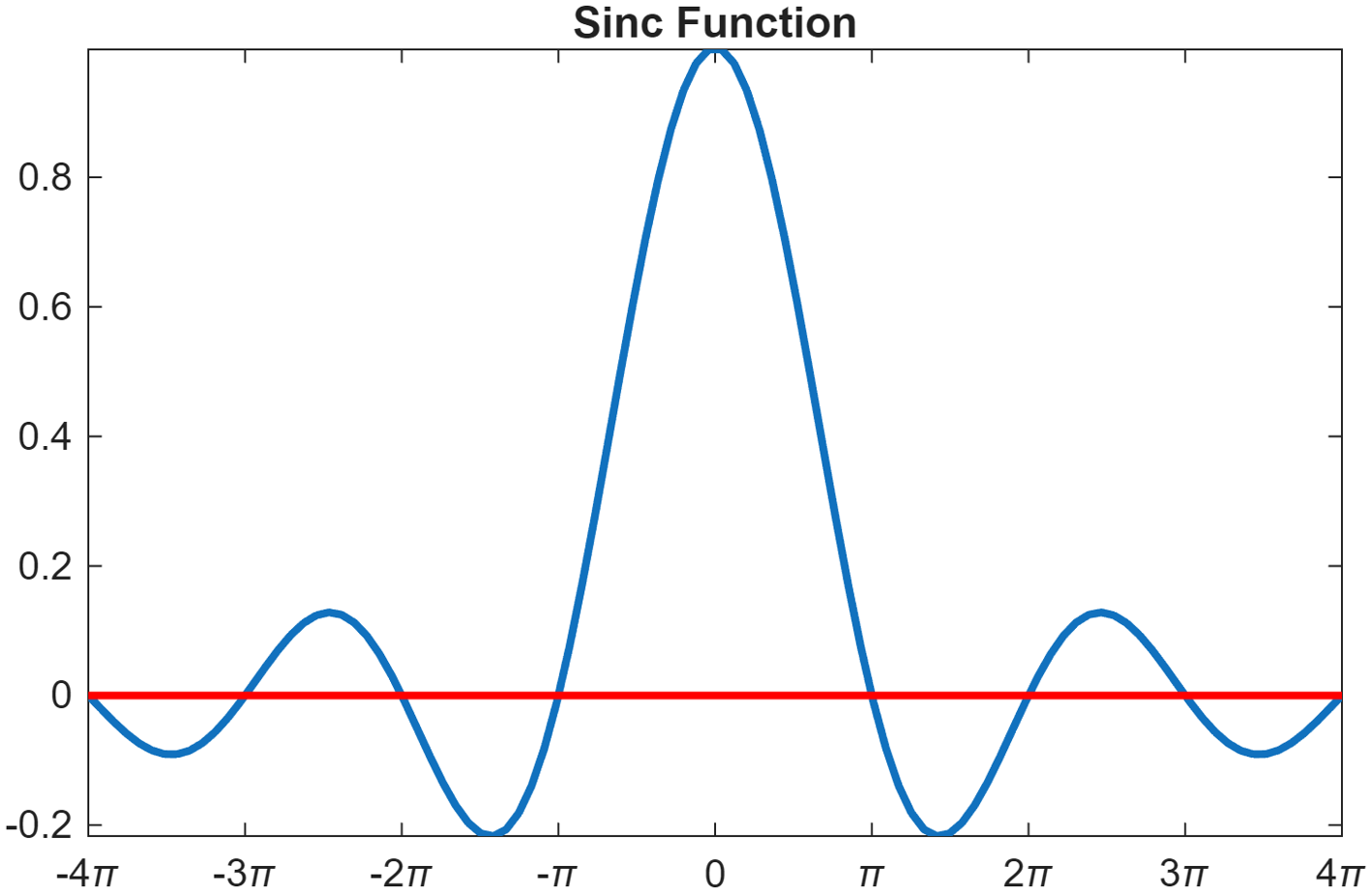
Fig. 2.6 Sinc function (\(\sin(x)/x\)) with logical vector indexing