2.5. For Loops
Here we introduce our first programming control construct. Control constructs determine which, if any, code is executed, and how many times the code is executed.
The for loop is considered a counting loop because the loop’s
declaration explicitly states the number of times that the loop will
execute.
2.5.1. Code Blocks
A code block is a set of commands grouped together to perform a task.
A code block may be a single command, or it may be a large section of
code. Different programming languages use different strategies to
identify a code block. In MATLAB, a code block is all of the code
between the initial line of the control construct (in this case,
for) and the keyword end.
2.5.2. For Loop Syntax
Here is the syntax of a for loop.
for idx = sequence
    code block
end
Here, sequence is a series of values (usually numbers in the form of a
row vector). Here is an example for loop. The variable k
sequentially gets the next value of the sequence each time the code
block runs. The variable k is 1 the first time through the loop. On
the second iteration, k is 2. During the third and final execution
of the loop, k is 3.
for k = 1:3
    disp(['Iteration: ',num2str(k)])
    disp(2*k)
end
The output from this loop is:
Iteration: 1
    2
Iteration: 2
    4
Iteration: 3
    6
2.5.3. Colon Sequences
The colon operator, as used in the previous example, is frequently used to create a sequence of numbers. The simplest colon operator usage takes two arguments and counts with a step size of one between the two arguments.
>> 1:5
ans =
    1   2   3   4   5
>> 3:7
ans =
    3   4   5   6   7
>> 1.5:4.5
ans =
    1.500    2.500    3.500    4.500
With three arguments, the first and third arguments specify the range as before, while the second argument gives the step size between items of the sequence.
>> 1:2:5
ans =
    1   3   5
>> -12:4:12
ans =
    -12   -8   -4    0    4    8   12
>> 0:0.5:3
ans =
    0   0.500   1.000   1.500   2.000   2.500   3.000
>> 3:-1:0
ans =
    3   2   1   0
2.5.4. Application of For Loops in MATLAB
A for loop is often used to iterate through a sequence of values or
items in an array, which is a cornerstone of numerical computing.
Although syntax differences exist, for loops are a significant
component of every computer programming language. However, as we will
see in Vectors and Matrices in MATLAB, and Functions Operating on Vectors, MATLAB does not always need a
for loop to iterate through an array. Element-wise arithmetic and
functions that operate on all of the values in a vector can be used
instead of a for loop.
In MATLAB, for loops are needed to execute algorithms with different
parameters or data sets, but not usually to apply a calculation to a
single data set. For example, one might use a for loop to plot a
series of data curves in a chart. Whereas, the data for each curve on
the chart might be generated using element-wise arithmetic and
vector-aware functions.
2.5.5. Fibonacci Sequence
The Fibonacci sequence of numbers is an exception to what was said earlier about not usually needing loops to generate data values in MATLAB because each value is derived from previously calculated values.
This is the first example where we will use an array (vector) to save
the results. We will discuss arrays more in Vectors and Matrices in MATLAB. We
preallocate the array with the zeros function.
The definition of the Fibonacci sequence is \(F_1 = 0\), \(F_2 = 1\), and \(F_i = F_{i-1} + F_{i-2}\) for \(i \geq 3\).
n = 50;  % number of terms
F = zeros(1,n);
% F(1) = 0 -- already set
F(2) = 1
for i = 3:n
    F(i) = F(i-1) + F(i-2);
end
2.5.6. First Plot
Plotting data will be discussed several times in the following chapters.
Here we will use a for loop to plot a sequence of points.
Start by entering the following in the Command Window:
>> plot(1, 2, 'o')
You should see a plot with a small circle at point \((x = 1, y = 2)\). If you plot another point, the first plot is replaced by the new one.
>> plot(2, 3, 'o')
If we want multiple plots on the same figure, we want to use hold on
to retain the same axis for all plots. When finished plotting, we issue
the hold off command so that future plots start over. It is common
to make the first plot to generate the graph and then use the
hold on command before adding new plots, but we can also use a loop
to make all of the plots after the hold on command.
Copy the code from Simple plot from a for Loop into a MATLAB script. The
appearance of the data points here are specified by the ’r*’ option,
which calls for red asterisks with no connecting line.
% File: firstPlot.m
%% Plot k^2 for k = 0 to 5
hold on
for k = 0:5
    plot(k, k^2, 'r*');
end
hold off
%% title and axis labels
title('Y = k^2')
xlabel('k')
ylabel('k^2')
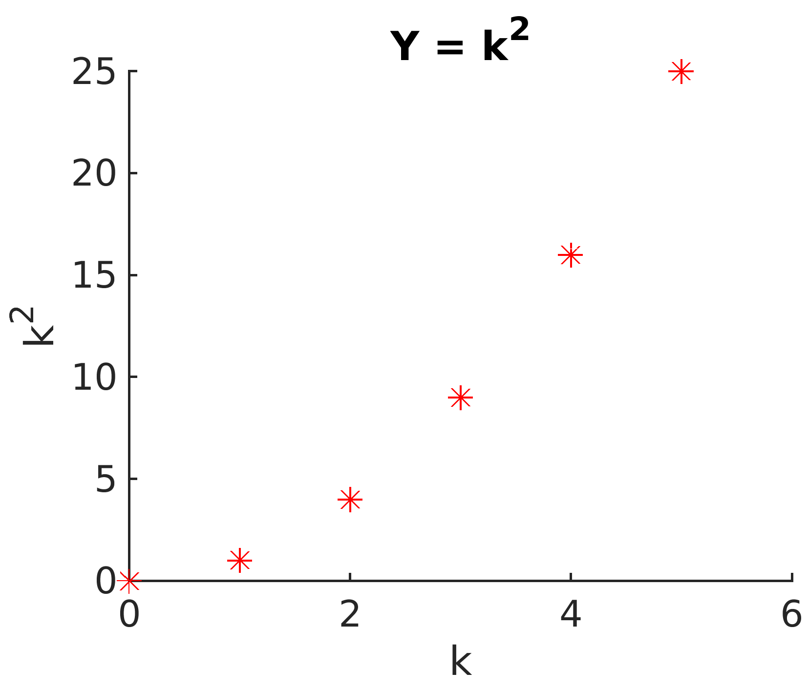
Fig. 2.2 Simple plot from a for Loop
A peak ahead
A better way to code Simple plot from a for Loop is to pass a sequence of points to one plot command as follows. We will discuss finding the sequence of \(y\) axis data points in Element-wise Arithmetic.
k = 0:5;
plot(k, k.^2, 'r*');
2.5.7. A Multi-line Plot
The next example shows using a for loop to plot
multiple lines. Note how MATLAB automatically uses a different color for
each curve. Also note the legend displayed at the top of the plot. We
discuss the details of plotting in the next chapter. Your plot should
look like
figure Fig. 2.3, except you should see colored plot
curves.
% File: multiline.m
% Multiline plot with a for loop
x = -1.5:0.1:1.5;
style = ["-", "--", "-."];
hold on
for k = 1:3
    plot(x, x.^k, style(k), 'LineWidth', 2)
end
axis tight
legend('y = x', 'y = x^2', 'y = x^3', 'Location', 'North')
hold off
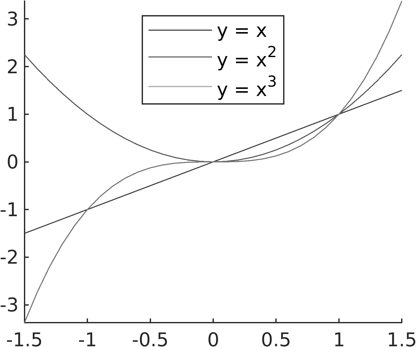
Fig. 2.3 Using a loop to plot multiple data curves on a plot.
