2.10. Importing Data Into MATLAB
Data files having several formats, such as TXT, CSV, XLS, and XLSX, can be imported into MATLAB both interactively and from commands. The latest list of supported import and export file formats is available on MathWorks’ website [FileFmts].
Search MathWorks’ website for videos and examples for importing spreadsheet data into MATLAB. In particular, the video at [Eigerman] and examples at [Quintero] are quite helpful.
2.10.1. Saving and Loading Workspace Data
You can save data from the workspace and load data into the workspace
using the save and load commands. These commands use files with
a .mat file name extension.
Create myData.mat containing current workspace variables.
>> save myData
You can selectively save individual variables instead of saving the entire
MATLAB workspace. Save x and y to someFile.mat.
>> save someFile x y
Load variables from myData.mat into the workspace.
>> load myData
2.10.2. Import Tool
The Import Tool is convenient for importing data from files with an intuitive graphical user interface. If the file has labels in the first row for each column, they will appear at the top of each column. You can also enter label names, see figure Fig. 2.7. The labels are used for naming the column vectors or table fields.
The Import Tool is available from the Home tab, labeled as “Import Data”. Notice the pull-down menu specifying “Output Type”. The choice of “Column vectors” yields similar vector data as we have previously used. Each column of data from the file is imported as a column vector.
Notice the two choices in the pull-down menu on the right side of the Import Tool labeled “Import Selection”. Options “Generate Script” and “Generate Function” can automate future imports.
Notice also how missing data will be handled. A pull-down menu offers choices. Replacing missing data with NaN (not a number) is often a good choice.
2.10.3. Reading Tables
We are most familiar with column vectors at this point, but it may not
always be the best choice. Importing data as a table is simpler to
perform from commands. The columns of a table can be converted to column
vectors if needed. Each table column doesn’t need to be of the same data
type. The data can be considered a series of observations (rows) over a
set of variables (columns). The sortrows function is used to sort
the data based on any table column, and the data in each row is kept
together.
The command for importing a table from a file is
readtable(’filename’). The columns of a table may be accessed as
column vectors using the notation of tableName.columnName.
2.10.4. Dealing with Missing Data
Data values that are missing show up as NaN (Not a Number. The MATLAB
function ismissing returns a logical vector showing where data is
missing. There are three basic ways to deal with missing data.
Ignore it: Some MATLAB statistics functions have an option
’omitnan’that will ignore any NaN values.Delete it: Setting a table row to
[\(\,\)]removes the data.Interpolate it: MATLAB has a function called
fillmissingthat will interpolate missing data in a vector between its neighboring data. Data Interpolation has more information about data interpolation.
The following tutorial shows example code for dealing with missing data.
It uses the file autompg.csv, which is a public domain dataset
available from the UCI Machine Learning
Repository [Dua:2019] as file
auto-mpg.data-original. The file contains six data values about 398
car models from 1970 to 1982. For our investigation, we will import only
the data columns for miles per gallon (mpg) in column 1, horsepower in
column 4, and weight in column 5. The most convenient way to import the
data into MATLAB is to use the Import Data Tool. Figure
Fig. 2.7 shows how column names are entered at the top
of each column and the desired columns are selected for import. The data
will be imported into a table, and any missing values will be replaced
with NaN (not a number).
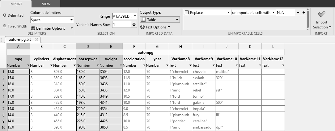
Fig. 2.7 The Import Data Tool is used to import desired data columns.
After the data is imported into a table, we verify the names of the
table fields. We will also save the data to make it easier to load
later. The saved file is autompg.mat.
>> autompg.Properties.VariableNames
ans =
  1x3 cell array
    {'mpg'}    {'horsepower'}    {'weight'}
>> save autompg
We will put our commands into a script, but use the “Run Section” button from the Edit tab to take things one step at a time.
First, we will check the three data fields to see if any data is
missing. The ismissing function will return a logical array, and the
nnz function will count how many values are missing.
% File: carTable.m
%% Dealing with missing data
%   Run this code one section at a time.

% Take a look at the part of the table
% autompg(1:4,:)

% count missing data
disp('missing MPG')
nnz(ismissing(autompg.mpg))
disp('missing Horsepower')
nnz(ismissing(autompg.horsepower))
disp('missing Weight')
nnz(ismissing(autompg.weight))
The horsepower field has six missing values.
missing MPG
ans =
     0
missing Weight
ans =
     0
missing Horsepower
ans =
     6
If we want to calculate statistics of the data, we can ignore the
missing data with the ’omitnan’ option. Most of the statistics
functions have this option. For more on statistics functions, see
Common Statistical Functions and check the documentation of the functions you
want to use.
%% Ignore missing data for mean

disp('mean Horsepower')
mean(autompg.horsepower, 'omitnan')
We may want to delete the rows with missing values. The following code also displays how many rows were deleted.
%% Delete rows with missing data

%  idx holds index of any rows with missing (NaN) values
idx = ismissing(autompg.horsepower);
autompg(idx,:) = [];    % remove rows missing values
disp('missing Horsepower')
nnz(idx)
missing Horsepower
ans =
     6
We would expect a negative correlation between horsepower and mpg values. A
quick scatter plot verifies this. We could use MATLAB’s corrcoef function
to calculate the correlation, but a scatter plot verifies what we already
expect. We only need to see the plot to verify the relationship, so we didn’t
bother to label the axes or give the plot a title. Figure Fig. 2.8
shows the scatter plot.
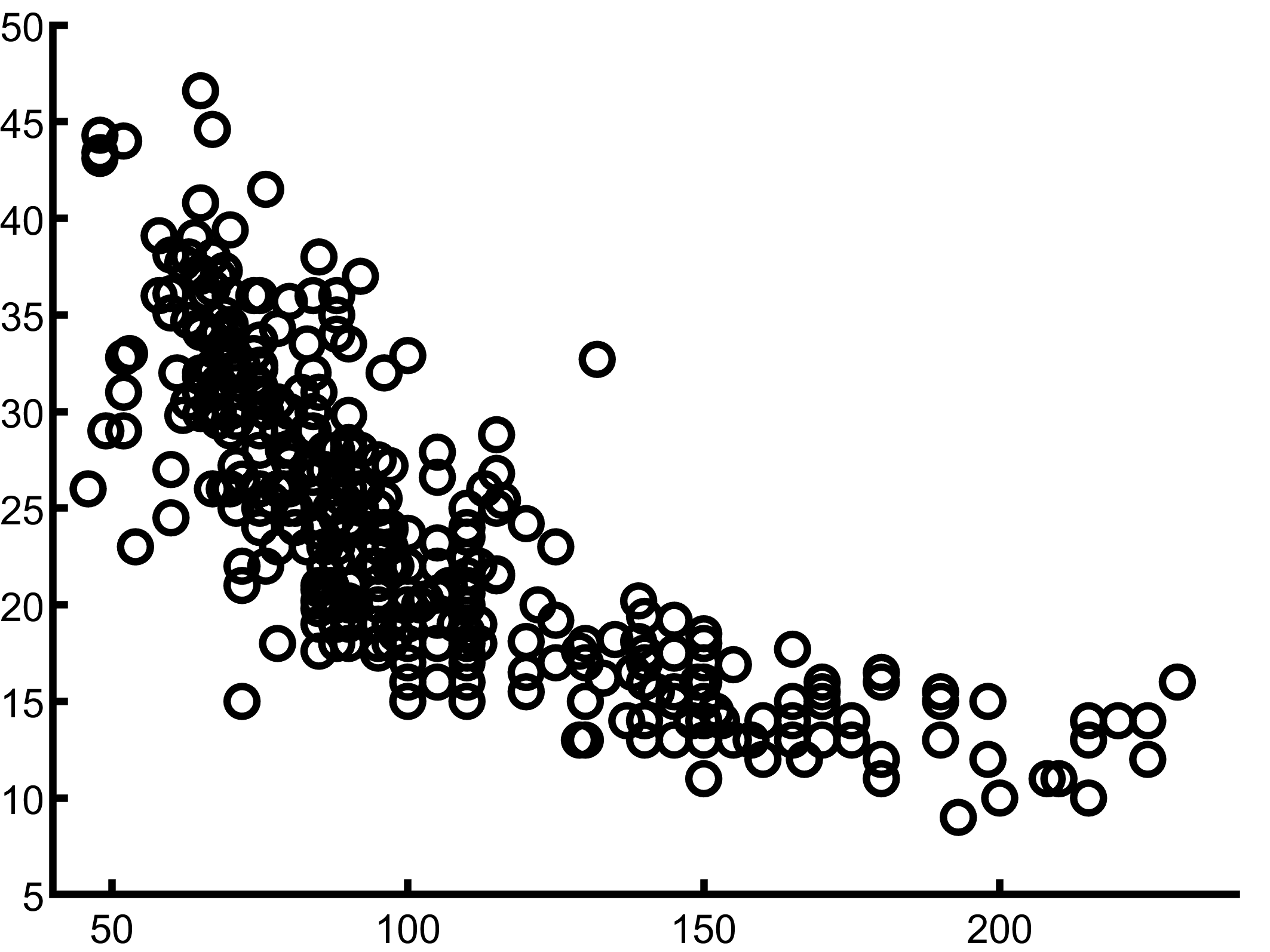
Fig. 2.8 Scatter plot of car horsepower against mpg
%% scatter plot to observe correlation between MPG
%  and Horsepower

scatter(autompg.horsepower, autompg.mpg)
Next, after reloading the data, we will use linear data interpolation to fill in the missing data. Since we know that the horsepower data is correlated to the mpg data, we can get reasonable results by sorting the data based on the mpg field. The long output (not shown) shows the values before and after the filled-in values and verifies that the estimates are reasonable.
Whether it is better to delete rows with missing values or use interpolation depends on the application, the data available, and your preferences.
%% Interpolate missing data
% re-load data with missing values
load autompg

% sort rows by MPG to group cars.
autompg = sortrows(autompg, 'mpg');
% find missing data
idx = find(ismissing(autompg.horsepower));
disp('missing data')
for i = idx'
    disp(autompg.horsepower(i-2:i+2))
    disp(' ')
end

% use linear interpolation
autompg.horsepower = ...
    fillmissing(autompg.horsepower, 'linear');
disp('interpolated data')
for i = idx'
    disp(autompg.horsepower(i-2:i+2))
    disp(' ')
end
2.10.5. Exporting Table Data
Use the writetable function to export a table to a delimited text
file or a spreadsheet.
>> writetable('myTable.csv');
By default, writetable uses the file name extension to determine the
appropriate output format.
Note
There is a lot more information about MATLAB tables that are not included here.
Now complete the tutorial in Working with Tables.
