8.6. Change of Basis and Difference Equations
When we wish to multiply \(\mathbf{A}^k\) by a vector (\(\mathbf{A}^k\bm{v}\)), we could diagonalize the matrix to find \(\mathbf{A}^k\) and then multiply by the vector. But there is another approach that also makes apparent the steady state of the system (when \(k\) goes to infinity). The change of basis method for computing \(\mathbf{A}^k\bm{v}\) has a particular application to difference equations, a commonly used model for discrete systems.
First, we must change the vector into a linear combination of the eigenvectors of \(\bf{A}\).
We call the procedure a change of basis because, as shown in figure Fig. 8.3, we use the eigenvectors as a new coordinate frame to describe the vector instead of the normal Cartesian basis vectors.
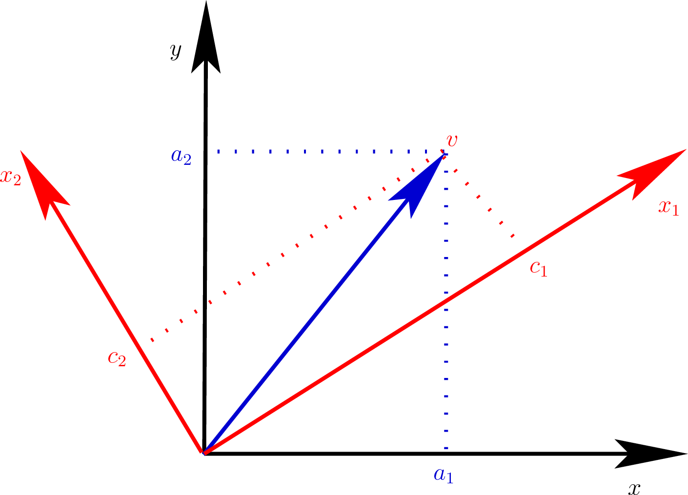
Fig. 8.3 Vector \(\bm{v}\) is changed from coordinates \((a_1, a_2)\) using the standard basis vectors to coordinates \((c_1, c_2)\) using the eigenvectors of \(\bf{A}\) as the basis vectors.
In matrix form, the vector \(\bm{v}\) is described as
Finding the linear coefficients is just a matter of solving a system of
linear equations: \(\bm{c} = \mathbf{X}^{-1}\bm{v}\), or in MATLAB:
c = X\v.
Now, we will take advantage of \(\mathbf{A\,X} = \mathbf{X\,\Lambda}\) along with \(\bm{v} = \mathbf{X}\,\bm{c}\) to multiply \(\bm{v}\) by powers of \(\bf{A}\),
Let’s illustrate this with an example. Consider the following matrix and its eigenvectors and eigenvalues. We will find \(\mathbf{A}^2 \bm{v}\) using the change of basis strategy, where \(\bm{v} = (3, 11)\) is changed to a linear combination of the eigenvectors.
>> A = [1 2; 5 4];
>> [X, L] = eig(A);
>> x1 = X(:,1);
>> x2 = X(:,2);
>> l1 = L(1,1);
>> l2 = L(2,2);
>> v = [3; 11];
>> c = X\v;
>> A^2 * v
ans =
   143
   361

% check with
% eigenvalues and eigenvectors
>> l1^2*c(1)*x1 + l2^2*c(2)*x2
ans =
   143
   361
To generalize, we can say that when
then
Note
Eigenvalues and eigenvectors are often complex, but the final result will be real (zero imaginary part).
8.6.1. Difference Equations
One of the main applications where you might want to compute the power of a matrix multiplied by a vector is for a difference equation, which is the discrete form of a differential equation. Difference equations are often used in the study of control systems, which is important to nearly every engineering discipline.
We can define a system’s state as a vector containing any set of desired conditions, e.g., position, velocity, acceleration, or anything else that describes a property of the system at an observation. The vector \(\bm{u}_0\) gives the system’s initial state. The matrix \(\mathbf{A}\) defines how the system’s state changes between observations.
The state of the system at the first observation is
After the second observation, it is
After \(k\) observations, it is
Applying equation (8.5) gives us an equation for the state of a system defined by a difference equation after \(k\) observations.
The eigenvalues and eigenvectors of \(\bf{A}\) are \(\lambda_i\) and \(\bm{x}_i\). The \(c\) coefficients are the elements of the vector \(\bm{c} = \mathbf{X}^{-1}\bm{u}_0\).
8.6.2. Application: Fibonacci Sequence
A simple application of a difference equation is the Fibonacci sequence of numbers, which is the sequence of numbers starting with 0 and 1, and continuing with each number being the sum of the previous two numbers: {0, 1, 1, 2, 3, 5, 8, 13, 21, \(\ldots\) }, \(\text{Fibonacci}(k) = \text{Fibonacci}(k-1) + \text{Fibonacci}(k-2)\). The Fibonacci sequence occurs in nature and is often fodder for programming problems using recursion and dynamic programming. Still, it can also be described as a difference equation, from which the change of basis method finds a closed-form solution known as Binet’s formula.
The state of the system here is a vector with \(\text{Fibonacci}(k)\) and \(\text{Fibonacci}(k - 1)\).
Let us use the change of basis strategy to compute \(\bm{F}(k)\) for any value of \(k\). One can quickly find the two eigenvalues.
However, the algebra to find the symbolic equation for the eigenvectors and the change of basis coefficients gets messy, but Chamberlain shows them in a blog post [CHAMBERLAIN16]. We can also let MATLAB compute the eigenvalues and eigenvectors using the Symbolic Math Toolbox.
[X, L] = eig(sym([1 1; 1 0]))
The eigenvectors are:
With elimination, we find the change of basis coefficients.
Then each Fibonacci number is given by the first value of the difference equation vector.
With this solution, \(\text{Fibonacci(0)} = 1\), but we observe that the eigenvector terms used are the same as the eigenvalues, so we are actually raising the eigenvalues to the \((k + 1)\) power. Thus, we can shift the terms and get a result with \(\text{Fibonacci(0)} = 0\).
The fibonacci function implements a closed-form (constant run time)
Fibonacci sequence. The function calculates integer values. The
round function returns values of integer data type instead of
floating point numbers.
function fib = fibonacci(k)
% FIBONACCI(k) - kth value of Fibonacci sequence from Binet's formula

    L = [(1 + sqrt(5))/2 0; 0 (1 - sqrt(5))/2];
    c = [1/sqrt(5); -1/sqrt(5)];
    % only need the first vector value
    fib = round(c(1)*L(1,1)^k + c(2)*L(2,2)^k);
end
8.6.3. Application: Markov Matrices
A Markov matrix is a stochastic matrix showing probabilities of something transitioning from one state to another in one observation period. There are many applications where things can be thought of as having one of a finite number of states. We often visualize state transition probabilities with a finite state machine (FSM) diagram. Then, we can build a Markov matrix from an FSM and make predictions. Markov models are named after the Russian mathematician Andrei Andreevich Markov (1856 - 1922).
Figure Fig. 8.4 shows a simple FSM with hypothetical odds for the weather on the next day given the current weather conditions.
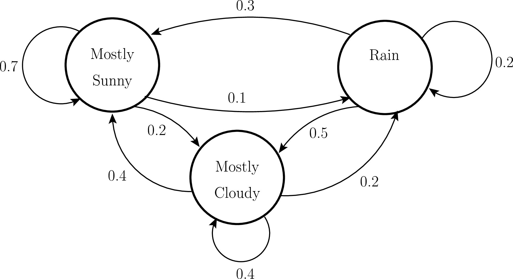
Fig. 8.4 Weather prediction finite state machine
We interpret the FSM diagram to say that if it is sunny today, there is a 70% chance that it will also be sunny tomorrow, a 20% chance that it will be cloudy tomorrow, and a 10% chance of rain tomorrow. Similarly, we can assign probabilities for tomorrow’s weather based on whether it is cloudy or raining today.
We put the transition probabilities into a Markov matrix. Since the values in the matrix are probabilities, each value is between zero and one. The columns represent the transition probabilities for starting in a given state. The sum of each column must be one. The rows represent the probabilities of the system being in a particular state on the next observation.
The columns and rows are ordered as sunny, cloudy, and rainy.
Matrix multiplication tells us the weather forecast for tomorrow if it is cloudy today.
>> M = [0.7, 0.4, 0.3; 0.2, 0.4, 0.5; 0.1, 0.2, 0.2]
M =
    0.7000    0.4000    0.3000
    0.2000    0.4000    0.5000
    0.1000    0.2000    0.2000
>> M * [0; 1; 0]
ans =
    0.4000      %  probability sunny
    0.4000      %  probability cloudy
    0.2000      %  probability rain
We need to raise \(\bf{M}\) to the \(k\) power to predict the weather in \(k\) days.
So if it is cloudy today, we can expect the following on the day after tomorrow.
>> M^2 * [0; 1; 0]
ans =
    0.5000     %  probability sunny
    0.3400     %  probability cloudy
    0.1600     %  probability rain
We will always see something interesting when we look at the eigenvalues of a Markov matrix. One eigenvalue will always be one, and the others will be less than one. So the forecast for future days converges and eventually becomes independent of the system’s current state.
>> [X, L] = eig(M)
X =
    0.8529    0.7961    0.1813
    0.4713   -0.5551   -0.7801
    0.2245   -0.2410    0.5988
L =
    1.0000         0         0
         0    0.3303         0
         0         0   -0.0303
The system’s steady state only depends on the eigenvector corresponding to the eigenvalue of value one. The other terms will go to zero in future observations.
>> c_sun = X\[1; 0; 0];
>> c_clouds = X\[0; 1; 0];
>> c_rain = X\[0; 0; 1];
>> steady_state = X(:,1)*c_sun(1)
steady_state =
    0.5507
    0.3043
    0.1449
>> steady_state = X(:,1)*c_clouds(1)
steady_state =
    0.5507
    0.3043
    0.1449
>> steady_state = X(:,1)*c_rain(1)
steady_state =
    0.5507
    0.3043
    0.1449
We can plot the forecast to see the convergence. The MarkovWeather
script shows the code for the change of basis calculation and plot of
the weather forecast. Each point in the 3-D plot is the probability of
sun, clouds, or rain for one day. The plot shows that the distant
forecast converges to the same probability regardless of today’s weather
conditions.
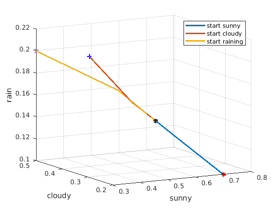
Fig. 8.5 A 3-D plot showing the Markov matrix forecast probabilities given that today is sunny, cloudy, or raining
% File: MarkovWeather.m
% Script showing the change of basis calculation for
% a Markov matrix.

M = [0.7, 0.4, 0.3; 0.2, 0.4, 0.5; 0.1, 0.2, 0.2];
[X, L] = eig(M);
l = diag(L);
% coefficients from initial conditions
c_sun = X\[1; 0; 0];
c_clouds = X\[0; 1; 0];
c_rain = X\[0; 0; 1];

N = 20;
F_sun = zeros(3, N);
F_clouds = zeros(3, N);
F_rain = zeros(3, N);
% build forecast for next N days
for k = 1:N
    F_sun(:,k) = c_sun(1)*X(:,1) + c_sun(2)*l(2)^k*X(:,2) ...
                + c_sun(3)*l(3)^k*X(:,3);
    F_clouds(:,k) = c_clouds(1)*X(:,1) + c_clouds(2)*l(2)^k*X(:,2) ...
                + c_clouds(3)*l(3)^k*X(:,3);
    F_rain(:,k) = c_rain(1)*X(:,1) + c_rain(2)*l(2)^k*X(:,2) ...
                + c_rain(3)*l(3)^k*X(:,3);
end

% plot probabilities for next 20 days
figure, hold on
plot3(F_sun(1,:), F_sun(2,:), F_sun(3,:))
plot3(F_clouds(1,:), F_clouds(2,:), F_clouds(3,:))
plot3(F_rain(1,:), F_rain(2,:), F_rain(3,:))
% mark starting points
plot3(F_sun(1,1), F_sun(2,1), F_sun(3,1), 'r', 'Marker', '*')
plot3(F_clouds(1,1), F_clouds(2,1), F_clouds(3,1), 'b', 'Marker', '+')
plot3(F_rain(1,1), F_rain(2,1), F_rain(3,1), 'm', 'Marker', 'x')
% mark final point
plot3(F_sun(1,N), F_sun(2,N), F_sun(3,N), 'k', 'Marker', '*')
grid on
xlabel('sunny')
ylabel('cloudy')
zlabel('rain')
legend({'start sunny', 'start cloudy', 'start raining'})
hold off
8.6.3.1. Markov Eigenvalues
Markov matrices must have an eigenvalue of one because of the steady state, \(\lim_{k\to\infty}\mathbf{M}^k\,\bm{v}\). By definition, the steady state is never zero or infinity, so there must be at least one eigenvalue of one and no eigenvalue greater than one.
Markov matrices have one eigenvalue equal to one because the columns add to one. Recall that the eigenvalues satisfy the requirement that the characteristic equation, \(\mathbf{C} = \mathbf{M} - \mathbf{I}\lambda\), is a singular matrix, which will occur when \(\lambda = 1\). Subtracting one from the diagonal elements makes each column sum to zero. So the rows are dependent because each row is \(-1\) times the sum of the other rows.
