8.3. Finding Eigenvalues and Eigenvectors
We will now discuss the mathematical relationships between a matrix and its eigenvalues and eigenvectors. The relationships lead to a simple strategy for calculating the eigenvalues and eigenvectors. Unfortunately, the simple approach is insufficient for matrices larger than \(2{\times}2\) because finding the eigenvalues requires factoring a polynomial. The quadratic equation is all that we need for a \(2{\times}2\) matrix; however, we don’t have good factoring procedures for larger polynomials. Still, the relationships and equations presented here are foundational for applying eigenvalues and eigenvectors to engineering problems and to the iterative algorithms used to find the eigenvalues and eigenvectors of a larger matrix.
Note
We present a simple iterative procedure in The Power Method that finds the largest and most important eigenvalue. Finding Eigenvectors describes how to find the eigenvector paired to a known eigenvalue. The more challenging task of computing all of the eigenvalues and eigenvectors of a matrix is referred to as the eigenvalue problem. Although eigenvalues were first discovered in the eighteenth century, the first successful solution to the eigenvalue problem was not developed until 1959 [UHLIG09]. Some of the significant milestones in the search for a solution to the eigenvalue problem are discussed in History of the Eigenvalue Problem. Orthogonal Matrix Factoring presents the first two iterative algorithms developed to solve the eigenvalue problem.
We will begin with the equation for eigenvectors and eigenvalues, and insert an identity matrix so that both sides have a matrix multiplied by a vector.
Then we rearrange the equation to find the characteristic eigenvalue equation.
We are not interested in the trivial solution to equation (8.1) where \(\bm{x} = \bm{0}\). Eigenvectors are defined to be nonzero vectors. The solution to the characteristic eigenvalue equation only exists when the columns of the matrix \(\mathbf{A} - \lambda\,\bf{I}\) form a linear combination with \(\bm{x}\) yielding the zero vector. The linear dependence of the columns of the characteristic equation means that it is singular, having a zero determinant.
8.3.1. Finding Eigenvalues
The \(n\) scalar eigenvalues, \(\{\lambda_1, \lambda_2, \ldots, \lambda_n\}\), can be viewed as the shift of the matrix’s main diagonal that will make the characteristic matrix singular. The Eigenvalues are found by subtracting \(\lambda\) along the diagonal and finding the set of \(\lambda\)s for which the determinant is zero.
Note
Since an eigenvalue shifts the matrix’s diagonal such that the matrix is singular, a singular matrix has a zero-valued eigenvalue for each dependent row or column. Diagonalization could be used to find the rank of a matrix, but the SVD calculation is faster Rank from the SVD).
The determinant yields a degree-\(n\) polynomial, which can be factored to find the eigenvalue roots.
For the generalized \(2{\times}2\) matrix, the coefficient of the \(\lambda\) term in the quadratic equation is the negative of the sum of the matrix diagonal (the trace), and the constant term is the determinant of the matrix.
The quadratic equation simplifies this result for \(2{\times}2\) matrices. We will define variables \(m\) as the mean of the diagonal elements and \(p\) as the determinant of the matrix. Then we have a simple equation for the two eigenvalues.
>> A
A =
    -6    -1
    -8    -4
>> eig(A)
ans =
    -8
    -2
>> m = -5;
>> p = 24 - 8; %  p = 16
>> l1 = m - sqrt(m^2 - p)
l1 =
    -8  %  l1 = -5 - 3
>> l2 = m + sqrt(25 - 16)
l2 =
    -2
There are two problems with finding the eigenvalues of matrices larger than \(2{\times}2\) using this procedure. First, calculating the determinant of a large matrix is slow. Secondly, we do not have acceptable methods for factoring larger polynomials. There are closed-form equations for degree-3 and degree-4 polynomials. However, unlike the quadratic equation, those equations are a mess—long and complicated. The polynomial factoring problem has confounded mathematicians for centuries. In 1823, Niels Henrik Abel proved that a direct algorithm cannot find the roots of a polynomial of degree greater than four [HADLOCK78]. Iterative algorithms are required to factor a polynomial of degree-5 or more, or to find the eigenvalues of a matrix larger than \(4{\times}4\).
In practice, iterative algorithms are used to find the eigenvalues of matrices larger than \(2{\times}2\). Orthogonal Matrix Factoring presents iterative algorithms for finding the full eigendecomposition, but the iterative power method may be used to find the largest eigenvalue.
8.3.2. The Power Method
The power method is a technique to compute the dominant eigenvalue of a matrix. Although it is an old and simple algorithm, it is still used in applications like Google’s PageRank algorithm, which requires only one eigenpair. The basic theory of how the algorithm works is based on the change of basis that occurs when a matrix is raised to a specified power and multiplied by a vector, \(\m{A}^k\bm{v}_0\). Diagonalization of the matrix simplifies the exponent calculation. It changes the basis of the coordinate system from a Euclidean coordinate system to one that uses the matrix’s eigenvectors as the basis vectors.
We can solve a system of linear equations to find the linear
coefficients: \(\bm{c} = \mathbf{X}^{-1}\bm{v}_0\), or in MATLAB:
c = X\v. However, the power method does not calculate the
coefficients.
With the change of basis, the eigenvalues are the only variables raised to the power \(k\). The term with the largest eigenvalue, \(\lambda_i\), will dominate the calculation. Terms associated with smaller eigenvalues contribute less when \(k\) becomes large. Since \(\abs{\lambda_1} > \abs{\lambda_2} > \cdots > \abs{\lambda_n}\), the limit involves only one eigenvalue.
The vector \(\bm{v}_0\) can be any vector of the same dimension as \(\m{A}\). If, for example, \(\m{A}\) is a \(2{\times}2\) matrix, then \(\bm{v}_0 = [1, 0]^T\) works. If \(k\) is large, the \(\bm{v}_k\) vectors are eigenvectors scaled by \(c_1 (\lambda_1)^k \norm{x_1}\). You will know if \(k\) is large enough or needs to be increased after calculating several eigenvalues for increasing values of \(k\). A simple equation determines the eigenvalue estimates. Equation (8.3) makes a substitution of \(\mathbf{A}\,\bm{v} = \lambda \bm{v}\) to show that the calculation finds the eigenvalue.
Note
Equation (8.3) is called the Rayleigh quotient after English physicist John William Rayleigh (1842–1919).
Here is an example eigenvalue calculation in the Command Window.
>> A = [4 -1; 5 -2];
>> eig(A)
ans =
     3
     1
>> vk = [1; 0];
>> for k = 1:10
vk = A*vk;
lambda = vk'*A*vk/(vk'*vk);
disp(lambda)
end
The first ten estimates of \(\lambda_1\) are {2.2927, 3.2760, 2.9122, 3.0298, 2.9901, 3.0033, 2.9989, 3.0004, 2.9999, 3.0000}. The rate at which the algorithm converges is proportional to the ratio of the two largest eigenvalues \(\abs{\lambda_1}/\abs{\lambda_2}\). In this small example, the convergence was fast, but \(\lambda_1\) and \(\lambda_2\) may have similar magnitudes for large matrices, so more iterations might be required before an accurate value is known.
8.3.3. Roots of a Polynomial by Eigenvalues
As illustrated in figure Fig. 8.2, an algorithm to find the eigenvalues of the matrix provides an iterative algorithm for factoring a polynomial. One should factor a polynomial by expressing it as a matrix, and then the polynomial’s roots will be the matrix’s eigenvalues.
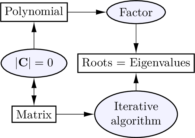
Fig. 8.2 The roots of a polynomial and the eigenvalues of a corresponding matrix are the same. It is faster and simpler to find the eigenvalues using an iterative algorithm rather than to factor a polynomial.
Let \(n\) be the degree of the polynomial, and let the row vector
\(p\) hold the polynomial coefficients. Then, build a shifted
identity matrix and use the coefficients in the first row. The MATLAB
commands below use the same algorithm as MATLAB’s roots function to
find the roots of the polynomial \(f(x) = x^3 - 4x^2 + x + 6 = 0\).
% n = degree of the polynomial
% coefficients
>> n = 3;
>> p = [1 -4 1 6];
>> A = diag(ones(n-1,1),-1)
A =
    0     0     0
    1     0     0
    0     1     0
>> A(1,:) = -p(2:n+1)./p(1)
A =
    4    -1    -6
    1     0     0
    0     1     0
>> r = eig(A)
r =
    3.0000
    2.0000
   -1.0000
The determinant of the characteristic equation of \(\bf{A}\) has the same coefficients as \(f(x)\), thus the eigenvalues of \(\m{A}\) are the roots of \(f(x)\).
The argument passed to the roots function is a row vector containing
the coefficients of the polynomial.
>> r = roots([1 -4 1 6])
r =
    3.0000
    2.0000
   -1.0000
The poly function is the inverse of roots:
>> poly(r)
ans =
    1.0000   -4.0000    1.0000    6.0000
8.3.4. Finding Eigenvectors
The eigenvectors, \(\bm{x}_i\) (one per eigenvalue), come from the null solution to the characteristic equation.
The eigenvectors can be found with elimination or with the null
function, which uses the SVD Null Space).
We will use elimination here to find the eigenvectors.
Add \(-1/2\) of row 1 to row 2 and then divide row 1 by \(4\):
The second row of zeros occurs because it is a singular matrix. So, we have a free variable, and can set one variable to any desired value (\(x_{1a} = 1\)).
Add \(2\) of row 1 to row 2 and then divide row 1 by \(-1\):
Note that MATLAB’s null and eig functions normalize the
eigenvector so that its length is one. The following example shows that
eigenvectors may be multiplied by a scalar to match the manual
calculations.
>> A = [2 2; 2 -1];
% the eigenvalues
>> l1 = -2; l2 = 3;
>> C1 = A - l1*eye(2)
C1 =
    4     2
    2     1
% normalized eigenvector
>> x1 = null(C1)
x1 =
   -0.4472
    0.8944
% scaled eigenvector
>> x1 = x1/x1(1)
x1 =
    1
   -2
>> C2 = A - l2*eye(2)
C2 =
   -1     2
    2    -4
% normalized eigenvector
>> x2 = null(C2)
x2 =
   -0.8944
   -0.4472
% scaled eigenvector
>> x2 = x2/x2(2)
x2 =
    2
    1
MATLAB has a function called eig that calculates a matrix’s
eigenvalues and eigenvectors. The results are returned as matrices. The
eigenvectors are the columns of X. The eigenvalues are on the
diagonal of L. The MATLAB command diag(L) will return the
eigenvalues as a row vector.
>> A = [2 2; 2 -1];
>> [X, L] = eig(A)
X =
    0.4472   -0.8944
   -0.8944   -0.4472
L =
   -2     0
    0     3
>> diag(L)
ans =
    -2
     3
Passing the matrix as a symbolic math variable to eig will show
eigenvectors that are not normalized.
>> [X, L] = eig(sym(A))
X =
[ -1/2, 2]
[    1, 1]
L =
[ -2, 0]
[  0, 3]
