11.1. Optimization
In this section, we consider numerical algorithms that find specific points that are either a root of a function (\(f(x_r) = 0\)) or locate a minimum value of the function (\({\arg\min_{x_m}}f(x)\)). We are primarily concerned with the simpler case where \(x\) is a scalar variable, but will use vector variables with some algorithms.
We also introduce an open-source framework for modeling optimization problems that allows for more flexibility and control in the specification of convex optimization problems.
11.1.1. Numerical Roots of a Function
See also
If analytic roots are needed, see Solve.
To find the numeric roots of a polynomial, see Roots of a Polynomial by Eigenvalues.
The roots of a function are where the function is equal to zero. The
numerical methods discussed here find a root of a function within a
specified range, even if the function is nonlinear. If the function
(equation) is a polynomial, then the roots function described in
Roots of a Polynomial by Eigenvalues can be used to find the roots.
See also
Three classic numerical algorithms find where a function evaluates to zero. The first function, Newton’s method, works best when we have an equation for the function and can take the derivative of the function. The other two algorithms only require that we can find or estimate the value of the function over a range of points.
11.1.1.1. Newton-Raphson Method
As illustrated in figure Fig. 11.1, the Newton-Raphson method, or just Newton’s method, uses lines that are tangent to the curve of a function to estimate where the function crosses the \(x\) axis.
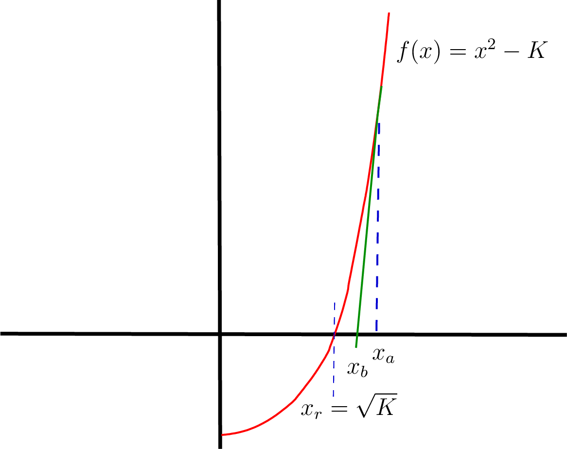
Fig. 11.1 The Newton-Raphson method extends a tangent line to the \(x\) axis to estimate a root value and repeats the process until the root is found within an allowed tolerance.
The algorithm evaluates the function at a sequence of estimates until the root is found.
Evaluate the function and its derivative at the first estimate, \(f(x_a)\) and \(f'(x_a)\).
The equation for a tangent line passing through the \(x\) axis is
\[f(x_a) - f'(x_a)(x_b - x_a) = 0.\]The estimate for the root is then
\[x_b = x_a - \frac{f(x_a)}{f'(x_a)}.\]If \(x_b\) is not close enough to the root at \(x_r\), then let \(x_a = x_b\) and repeat the steps.
The illustration in figure Fig. 11.1 shows finding \(x_r = \sqrt{K}\). Let \(f(x) = x^2 - K\), then \(f'(x) = 2\,x\).
The newtSqrt function uses the Newton-Raphson method to find the
square root of a number.
function x = newtSqrt(K)
% NEWTSQRT - Square root using the Newton-Raphson method
%   x = newtQqrt(K) returns the square root of K
%                   when K is a real number, K > 0.

    if ~isreal(K) || K < 0
        error('K must be a real, positive number.')
    end
    tol = 1e-7; % reduce tolerance for more accuracy
    x = K;      % starting point
    while abs(x^2 - K) > tol
        x = (x + K/x)/2;
    end
>> newtSqrt(64)
ans =
    8.0000
>> newtSqrt(0.5)
ans =
    0.7071
In the case of a polynomial function such as the square root function,
one can also use the roots function described in Roots of a Polynomial by Eigenvalues.
For example, the square root of 64 could be found as follows.
>> roots([1 0 -64])
ans =
    8.0000
   -8.0000
We can also write a general function to implement the Newton-Raphson
method for finding the roots of a function. The newtRoot function
needs an anonymous function to evaluate the function and its derivative.
function x = newtRoot(f, df, start)
% NEWTROOT - Find a root of the function f using
%            the Newton-Raphson method.
%   x = newtQqrt(f, df , start) returns x, where f(x) = 0.
%       f - function, df - derivative of function,
%       start - initial x value to evaluate.
%   Tip: First plot f(x) with fplot and pick a start value where
%        the slope of f(start) points towards f(x) = 0.


    tol = 1e-7; % reduce tolerance for more accuracy
    x = start;  % starting point
    while abs(f(x)) > tol
        d = df(x);
        d(d==0) = eps; % prevent divide by 0
        x = x - f(x)/d;
    end
>> newtRoot((@(x) cos(x) + sin(x) - 0.5), ...
    (@(x) cos(x) - sin(x)), 1.5)
ans =
    1.9948
>> cos(ans) + sin(ans) - 0.5
ans =
   -1.4411e-13
11.1.1.2. Bisection Method
The bisection algorithm converges slowly to find the root of a function, but it has the advantage that it will always find a root. The bisection algorithm requires two \(x\) values, \(a\) and \(b\), where the function crosses the \(x\) axis between the two points. As shown in figure Fig. 11.2, a new point is found that is halfway between the points.
If \(c\) is not within the allowed tolerance of the root, then one
of the endpoints is changed to \(c\) such that we have a new,
smaller range spanning the \(x\) axis. The bisectRoot function
implements the bisection root-finding algorithm.
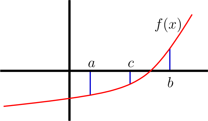
Fig. 11.2 The bisection algorithm cuts the range between \(a\) and \(b\) in half until the root is found midway between \(a\) and \(b\).
function x = bisectRoot(f, a, b)
% BISECTROOT  find root of function f(x), where a <= x <= b.
%    x = bisectRoot(f, a, b)
%    f - a function handle
%    sign(f(a)) not equal to sign(f(b))

    tol = 1e-7; % reduce tolerance for more accuracy
    if sign(f(a)) == sign(f(b))
        error('sign of f(a) and f(b) must be different.')
    end
    if f(a) > 0 % swap end points f(a) < 0, f(b) > 0
        c = a; a = b; b = c;
    end
    c = (a + b)/2; fc = f(c);
    while abs(fc) > tol && abs(b - a) > tol
        if fc < 0
            a = c;
        else
            b = c;
        end
        c = (a + b)/2; fc = f(c);
    end
    x = c;
>> f = @(x) x^2 - 64;
>> bisectRoot(f, 5, 10)
ans =
    8.0000
>> bisectRoot((@(x) cos(x) - 0.5), 0, pi/2)
ans =
    1.0472
11.1.1.3. Secant Method
The secant algorithm is similar to the bisection algorithm in that we
consider a range of \(x\) values that get smaller after each
iteration of the algorithm. As illustrated in figure
Fig. 11.3, the secant method finds its next point of
consideration by making a line between the endpoints and finding where
the line crosses the \(x\) axis. The secantRoot function
implements the secant root-finding algorithm.
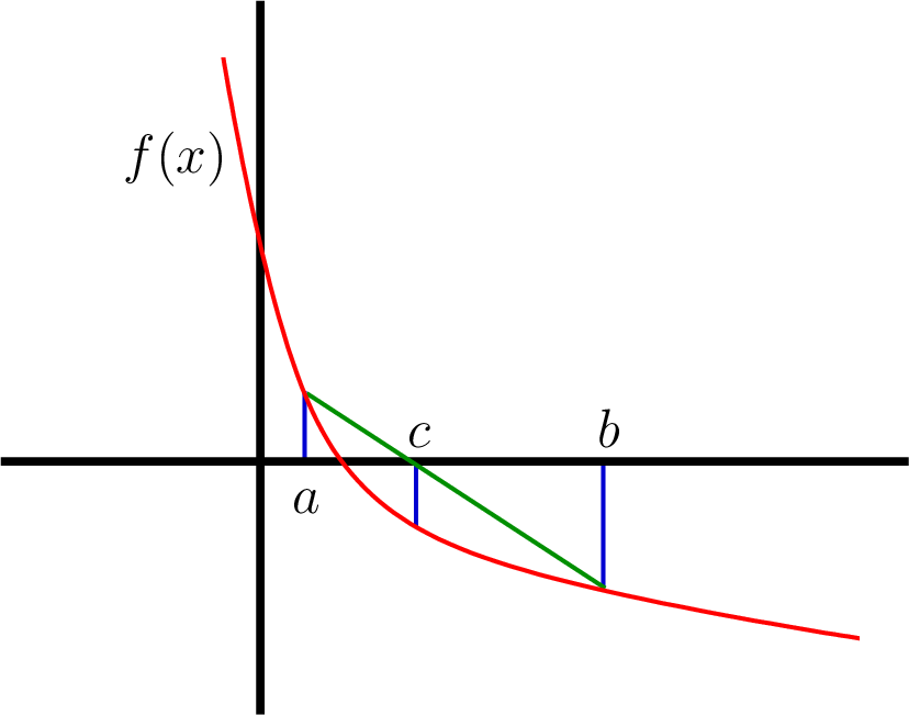
Fig. 11.3 The secant algorithm cuts the range between \(a\) and \(b\) by finding a point \(c\) where a line between \(f(a)\) and \(f(b)\) crosses the \(x\) axis. The range is repeatedly reduced until \(f(c)\) is within an accepted tolerance.
function x = secantRoot(f, a, b)
% SECANTROOT  find root of function f(x), where a <= x <= b.
%    x = secantRoot(f, a, b)
%    f - a function handle
%    sign(f(a)) not equal to sign(f(b))

    tol = 1e-7; % reduce tolerance for more accuracy
    if sign(f(a)) == sign(f(b))
        error('sign of f(a) and f(b) must be different.')
    end
    if a > b % swap end points a < b
        c = a; a = b; b = c;
    end
    sign_a = sign(f(a));
    c = a + abs(f(a)*(b - a)/(f(b) - f(a)));
    fc = f(c);
    while abs(fc) > tol && abs(b - a) > tol
        if sign(fc) == sign_a
            a = c;
        else
            b = c;
        end
        c = a + abs(f(a)*(b - a)/(f(b) - f(a)));
        fc = f(c);
    end
    x = c;
>> f = @(x) x^2 - 64;
>> secantRoot(f, 5, 10)
ans =
    8.0000
>> secantRoot((@(x) cos(x) - 0.3), 0, pi/2)
ans =
    1.2661
>> secantRoot((@(x) sin(x) - 0.3), 0, pi/2)
ans =
    0.3047
11.1.1.4. Fzero
MATLAB has a function called fzero that uses numerical methods to
find a root of a function. It uses an algorithm that is a combination of
the bisection and secant methods.
The arguments passed to fzero are a function handle and a row vector
with the range of values to search. The function should be positive at
one of the vector values and negative at the other value. The example in
figure Fig. 11.4 uses the fplot function to help find
good values to use. The plot displays values of the function over a
range to see where it crosses the \(x\) axis.
>> f = @(x) cos(x) - x;
>> fplot(f, [0 pi/2])
>> grid on
>> fzero(f, [0.5 1])
ans =
    0.7391
>> f(ans)
ans =
1.1102e-16
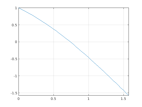
Fig. 11.4 The plot from fplot helps one select the search range to pass to
fzero.
11.1.2. Finding a Minimum
Finding a minimum value of a function can be a harder problem than finding a function root (where the function is zero). Ideally, we would like to use analytic techniques to find the optimal (minimal) values. We learn from calculus that a minimum or maximum of a function occurs where the first derivative is zero. Indeed, derivatives are always important in finding where a minimum occurs. However, when the function is nonlinear and involves several variables, finding an analytic solution may not be possible, so we use numerical search algorithms instead.
There are several numerical algorithms for finding where a minimum occurs. Our coverage is restricted to algorithms operating on convex regions. By convex, we mean like a bowl. If we pour water over a convex surface, the minimum point is where the water stops flowing and begins to fill the bowl-like surface. Some functions are strictly convex, while others have local minimum points that are not the global minimum point. In the latter case, we need to restrict the search domain. MATLAB includes two minimum search functions that are discussed below. MathWorks also sells an Optimization Toolbox with enhanced algorithms not discussed here. There are also third-party and open source resources with impressive capabilities. One such resource is discussed below in CVX for Disciplined Convex Programming.
The mathematics behind how these algorithms work is beyond the scope of
this text. Thus, we focus on what the algorithms can do and how to use
them. As with algorithms that find a root of a function, the minimum
search algorithms call a function passed as an argument many times as
they search for the minimum value. The first of MATLAB’s two minimum
search functions is fminbnd, which finds the minimum of functions of
one variable. The second function, fminsearch, handles functions
with multiple variables.
11.1.2.1. Fminbnd
The MATLAB function x = fminbnd(f, x1, x2) returns the minimum value
of function \(f(x)\) in the range \(x_1 < x < x_2\). The
algorithm is based on golden section search and parabolic interpolation
and is described in a book co-authored by MathWorks’ chief mathematician
and co-founder, Cleve Moler [FORSYTHE76]. We use
fminbnd to find the minimum value of a function in figure
Fig. 11.5.
>> f = @(x) x.^2-sin(x)-2*x;
>> fplot(f, [0 pi])
>> grid on
>> fminbnd(f, 1, 1.5)
ans =
    1.1871
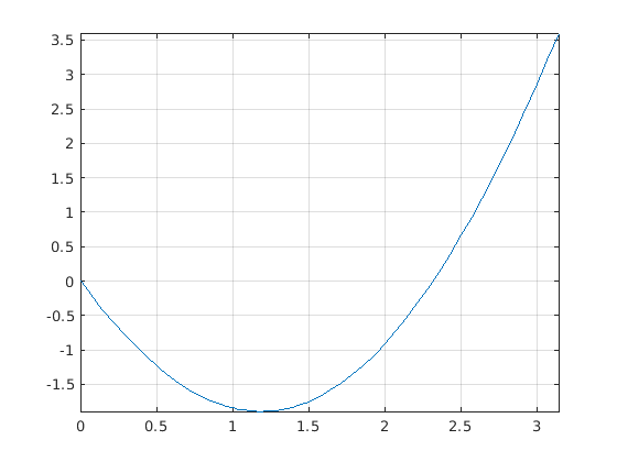
Fig. 11.5 The plot from fplot shows that the minimum value of the function
\(f(x) = x^2 - \sin(x) - 2\,x\) is between 1 and 1.5, fminbnd then
searched the region to find the location of the minimum value.
11.1.2.2. Fminsearch
The MATLAB function fminsearch uses the Nelder-Mead simplex search
method [LAGARIAS98] to find the minimum value of a
function of one or more variables. The fminsearch function takes a
starting point for the search rather than a search range. The starting
point may be a scalar or an array (vector) for multi-variable searches.
Best results are achieved when the supplied starting point is close to
the minimum location.
The fminsearch1 script evaluates a function that defines a
3-dimensional surface to find the location of its minimum. The overall
shape of the surface is a bowl, but with local hills and valleys from a
cosine term. The surface is plotted in figure Fig. 11.6
along with output from the script.
% File: fminsearch1.m
% fminsearch example
f = @(x) x(1).^2 + x(2).^2 + 10*cos(x(1).*x(2));
m = fminsearch(f, [1 1]);
disp(['min at: ', num2str(m)]);
disp(['min value: ', num2str(f(m))]);
% plot it now
g = @(x, y) x.^2 + y.^2 + 10*cos(x.*y);
[X, Y] = meshgrid(linspace(-5, 5, 50), linspace(-5, 5, 50));
Z = g(X, Y); surf(X, Y, Z)
min at: 1.7147    1.7147
min value: -3.9175
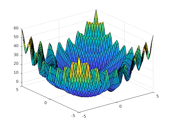
Fig. 11.6 Surface searched by fminsearch to find the location of the minimum
value. The output of the fminsearch1 script shows the location and value
of the minimum.
A common strategy for using fminsearch is to define a function
handle that computes an error function to minimize. For example, we can
define an error function as the distance between a desired robot end
effector location and a forward kinematics calculation. Then
fminsearch can calculate the inverse kinematics problem to find the
joint angles needed to position the robot end effector at the specified
location. The forward kinematics calculation uses matrix multiplication
to calculate the end position of a serial-link robotic arm. An analytic
inverse kinematic solution may be possible for robots with only a few
joints. However, more complex robots often require numerical methods to
find the desired joint angles. The starting point value is critical for
finding the desired joint angles because multiple joint angle sets can
position the robot arm at the same location.
Script fminsearch2 shows a simple example of a joint angle search
for a serial-link robot arm, as shown in figure Fig. 6.17.
The robot arm has two joints and two rigid arm segments (a and
b). The minimized function returns the length of the error vector
between a forward kinematic calculation and the desired location of the
end effector. The forward kinematic calculations use functions from
Peter Corke’s Spatial Math Toolbox [CORKE20] to
produce two-dimensional homogeneous coordinate rotation and translation
matrices as used in Coordinate Transformations in 2-D.
% File: fminsearch2.m
% Script using fminsearch for inverse kinematics
% calculation of a 2-joint robot arm.
E = [5.4 4.3]';
error = @(Q) norm(E - fwdKin(Q));
Qmin = fminsearch(error, [0 0]);
disp(['Q = ', num2str(Qmin)]);
disp(['Position = ', num2str(fwdKin(Qmin)')]);

function P = fwdKin(Q)
    a = 5; b = 2;
    PB = trot2(Q(1)) * transl2(a,0) * trot2(Q(2)) * transl2(b,0);
    P = PB(1:2,3);
end
The output of the script is the joint angles for the robot and forward kinematic calculation of the end effector position with those joint angles.
>> fminsearch2
Q = 0.56764      0.3695
Position = 5.4         4.3
11.1.3. CVX for Disciplined Convex Programming
CVX [1] is a MATLAB-based modeling system for convex optimization. CVX
lets users specify constraints and objectives using standard MATLAB
syntax, which provides flexibility and control in specifying
optimization problems. Commands to specify and constrain the problem are
placed between cvx_begin and cvx_end statements. CVX defines a
set of commands and functions that can be used to describe the
optimization problem. Most applications of CVX will include a call to
either the minimize or maximize
function [CVX20].
An example illustrates how to use CVX. Recall from The Preferred Under-determined Solution that the preferred solution to an under-determined system of equations is one that minimizes the \(l_2\)-norm of \(\bm{x}\), which is found with strategies based on projection equations and using either the SVD or QR decomposition. In addition to minimizing the length of \(\bm{x}\), it is desired that \(\bm{x}\) be sparse, having several zeros. The left-divide operator returns a solution with \((n-r)\) zeros by zeroing out matrix columns before finding a solution using the QR method (QR and Under-determined Systems, and Left-Divide of Under-determined Systems). It is also known that minimizing the \(l_1\)-norm tends to yield a sparse solution. We turn to CVX to replace the inherent \(l_2\)-norm we get from our projection equations with an \(l_1\)-norm. CVX gives a result that also contains zeros, but has a smaller \(l_1\)-norm than the left-divide solution.
>> A = [2 4 20 3 16;
        5 17 2 20 17;
       19 11 9 1 18];
>> b = [5; 20; 13];
>> cvx_begin
>>  variable x(5);
>>  minimize( norm(x, 1) );
>>  subject to
>>      A*x == b;
>> cvx_end
>> x
x =
   -0.0000
    1.1384
    0.0000
    0.0103
    0.0260
>> A*x
ans =
    5.0000
   20.0000
   13.0000
Footnote:
