17.5. Discrete 2D Fourier Transform of Images
Two dimensional signals, such as spatial domain images, are converted to the
frequency domain in a similar manner as one dimensional signals. Let the
image data be called  ; where
  represents the rows
and has range
represents the rows
and has range ![[0, 1, 2, \ldots M-1]](../_images/math/fd1783ab83f7c4795dbe483e4eb9fb34c186215c.png) ; and
; and  represents the
columns and has range
represents the
columns and has range ![[0, 1, 2, \ldots N-1]](../_images/math/52701b866e01e9c6160e49eb3d154568629b34ab.png) . Then the frequency
domain representation of the image is
. Then the frequency
domain representation of the image is  ; where likewise,
 and
and  range from 0 to M-1 and 0 to N-1.
-
Discrete Fourier Transform 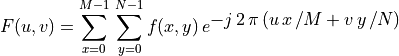
-
Inverse Discrete Fourier Transform 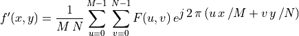
Note
- In MATLAB, x and u range from 1 to M, not 0 to M-1.
- In MATLAB, y and v range from 1 to N, not 0 to N-1.
- Like with the DFT, there is some variation in the literature about the
multiplier in front of the sum. Some people put
 in
the 2D-DFT equation. Others put it in the 2D-IDFT equation. This is what
MATLAB does. Other still put
in
the 2D-DFT equation. Others put it in the 2D-IDFT equation. This is what
MATLAB does. Other still put  in both
equations.
in both
equations.
-
Properties ![F[u, v]](../_images/math/87ada4a994eb90aae9be0226043cf4ef52191776.png) is complex, discrete, and periodic.
is complex, discrete, and periodic.The range indices may be regarded as spanning the complex exponential basis function from 0 to
 . In relation to frequencies,
we prefer to label the negative values from
. In relation to frequencies,
we prefer to label the negative values from  to 0, rather
than from
to 0, rather
than from  to
to - u = 0 to M/2 - 1 are positive frequencies.
- u = M/2 to M-1 are negative frequencies.
- v = 0 to N/2 - 1 are positive frequencies.
- v = N/2 to N-1 are negative frequencies.
- MATLAB has a function called
fftshiftthat is often used when plotting in the frequency domain. To display the plot so that 0 is at the center, instead of, it is necessary to
shift the x and y axis.
For best result when using numerical software, such as MATLAB, choose M and N to be a power of 2 (2, 4, 8, 16, 32, 64, 128, 256, 512 …). The reason for this is explained when the
fftfunction is discussed. For both images and one dimensional signals that are not a power of 2, zeros may be added to the end of the data to reach the next power of 2.For the same reasons discussed with regard to the DFT, 2D-DFT data is periodic in both the
and directions.
Images in the frequency domain are periodic
17.5.1. Units and Intuitive Feel for Frequency in Images
Because 1D discrete signals come from analog (continuous) signals, sampled
at a set rate, the coefficients may be matched to a frequencies in Hz. Images, being in the spatial domain, are slightly
different. We often reference the coefficients to the frequency of the
complex exponential basis function in radians; but usually, no value or
units are given for the frequencies. We can label one pixel-cycle as
a set of linear image pixels that correlate to a periodic function, such as
 ,
,  , or square wave, traversing one cycle. The set of
pixels in a pixel-cycle should show periodicity with respect to relatively
light and dark pixels. A pixel-cycle might appear as the set of pixels
showing a quarter cycle of white, followed by half cycle of black, followed
by another quarter cycle of white (or vice versa), or it might be a full
half cycle of either black or white followed by a full half cycle of the
other. Of course, pixel-cycles can also occur in shades of gray. With this
definition of linear pixel-cycles, we can view the image frequency in terms
of pixel-cycles per image. Keep in mind that each frequency coefficient
represents both a horizontal and a vertical frequency.
, or square wave, traversing one cycle. The set of
pixels in a pixel-cycle should show periodicity with respect to relatively
light and dark pixels. A pixel-cycle might appear as the set of pixels
showing a quarter cycle of white, followed by half cycle of black, followed
by another quarter cycle of white (or vice versa), or it might be a full
half cycle of either black or white followed by a full half cycle of the
other. Of course, pixel-cycles can also occur in shades of gray. With this
definition of linear pixel-cycles, we can view the image frequency in terms
of pixel-cycles per image. Keep in mind that each frequency coefficient
represents both a horizontal and a vertical frequency.
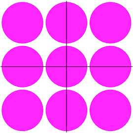
The pixel-cycles per image may be seen in the image below. This is a 5x5 grid of 8x8 binary images showing positive image frequencies. The image in the upper left represents the DC component (pixel intensity average) with no pixel-cycles. The next image to the right shows one horizontal pixel-cycle. The image below the DC image shows one vertical pixel-cycle. The images on the diagonal show images with both horizontal and vertical pixel-cycles. The image in the lower right shows the highest frequencies possible - 4 horizontal and 4 vertical pixel-cycles per image. The 8x8 pixels in the lower right image change between black and white at every pixel, thus every two pixels represents a pixel-cycle.
Note: Think of the length of pixel-cycle like the wavelength of any periodic function. Some pixel-cycles might be very long showing a low frequency. The minimum number of pixels in a pixel-cycle are two, such as one black and one white. Thus, no more than N/2 horizontal image cycles, and no more than M/2 vertical image cycles may appear in an image.
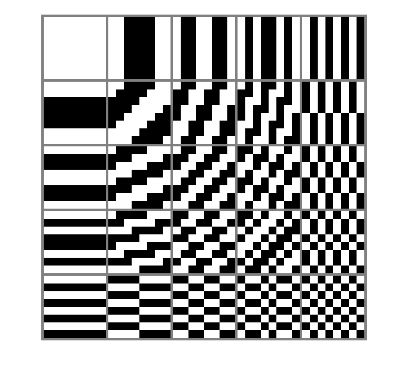
Grid of binay spatial domain images with positive frequencies. Here, N
and M = 8, so we show the DC componet and 4 ( basis function).
positive frequencies.
FYI …
Each 8x8 image in the image frequency grid was assigned horizontal
and vertical frequency values  then the pixel values were
calculated as
then the pixel values were
calculated as 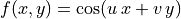 . Then the pixels were
converted to binary - 0 or 1. Actually, it was just little harder to make
the images because an 8x8 image looks very small on the computer screen.
Each image is actually 128x128 pixels with each 16x16 set of pixels
grouped together to appear as one pixel. The images are shown in binary
because it easier to see the pixel-cycles in binary.
. Then the pixels were
converted to binary - 0 or 1. Actually, it was just little harder to make
the images because an 8x8 image looks very small on the computer screen.
Each image is actually 128x128 pixels with each 16x16 set of pixels
grouped together to appear as one pixel. The images are shown in binary
because it easier to see the pixel-cycles in binary.
Something to think about
As we talk about frequencies of images, we are only concerning ourselves
with the indexes of the 2D-DFT coefficients. How does
both the magnitude and phase impact of the 2D-DFT coefficients affect
the appearance of the spatial domain image?
-
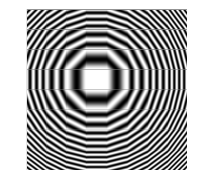
Just for fun .. Here is another frequency grid image. This one shows the negative frequencies also.
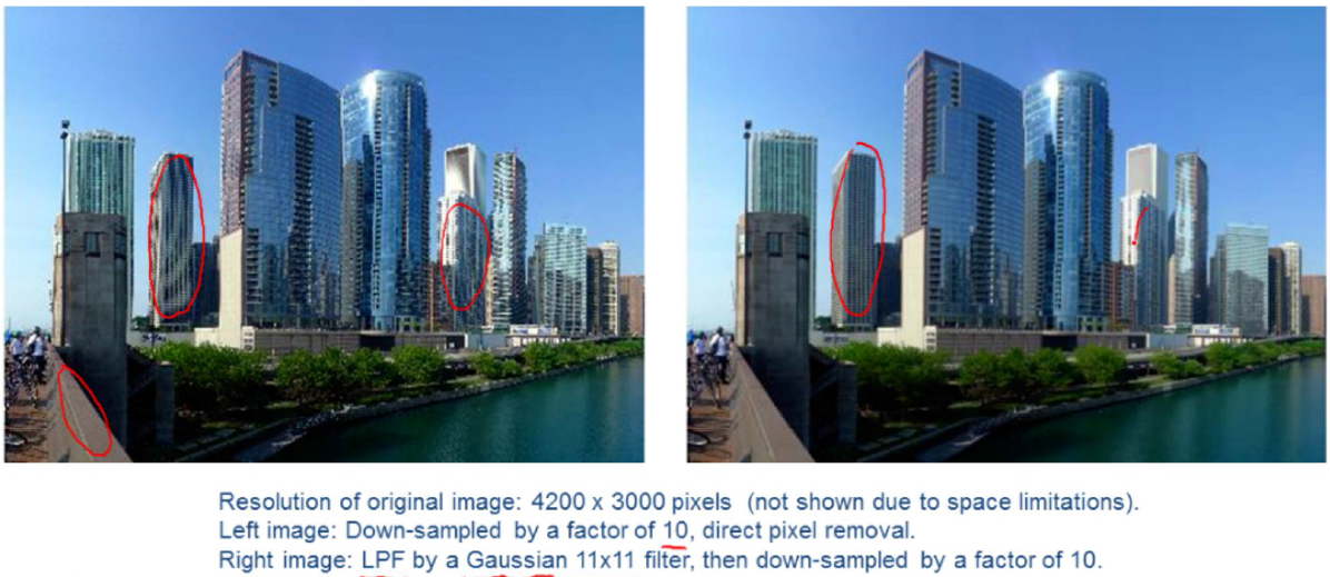
17.5.2. Aliasing and Nyquist Theorem
Since cameras acquire digital images very differently than one dimensional signals are acquired and sampled, we don’t need to be concerned about aliasing in an original image - at least not for this course. That said, one should assume that digital images fill the full spectrum available, thus aliasing can occur as a result of image processing. This is particularly a concern when reducing the size of an image. One should always low-pass filter an image before down sampling it (deleting rows and columns of data). Figure 5.16 (page 98) of the text book shows some nice pictures of image aliasing resulting from improper down sampling of an image. High frequency parallel lines (small pixel-cycle length) appear distorted when aliasing occurs.
Below is another picture showing image aliasing and how it can be avoided by filtering first. This picture comes from the lecture slides from the Coursera MOOC on Digital Image and Video Processing taught by Aggelos Katsaggelos of Northwesten University. Aliasing can be clearly seen in the circled building on the left side of the image.