17.4. Discrete 1D Fourier Transform
The continuous time signal  is sampled every
  seconds
to obtain the discrete time signal
seconds
to obtain the discrete time signal  .
Discrete Fourier transforms (DFT) are computed over a sample window of
.
Discrete Fourier transforms (DFT) are computed over a sample window of
 samples, which can span be the entire signal or a portion of it.
-
Discrete 1D Fourier Transform 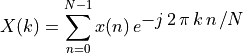
-
Inverse Discrete Fourier Transform 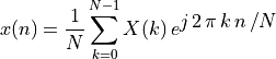
Note
- In MATLAB, k and n range from 1 to N, not 0 to N-1.
- There is some variation in the literature about the multiplier in
front of the sum. Some people put
 in the DFT
equation. Others put it in the IDFT equation. This is what MATLAB
does. Other still put
in the DFT
equation. Others put it in the IDFT equation. This is what MATLAB
does. Other still put  in both.
-
Properties ![X[k]](../_images/math/c1a3f86faacc9485e460ec02f9cbc5b570e40a1a.png) is complex, discrete, and periodic.
is complex, discrete, and periodic.The range of k from 0 to N-1 may be regarded as spanning the complex exponential basis function from 0 to
 . In relation to
frequencies, we prefer to view the values from
. In relation to
frequencies, we prefer to view the values from  to
as from
to
as from  to 0.
to 0.- k = 0 to N/2 are positive frequencies.
- k = N/2 to N-1 are negative frequencies.
- MATLAB has a function called
fftshiftthat is often used when plotting in the frequency domain. It is necessary to shift the x-axis to display the plot so that 0 is at the center, instead of or N/2 being the center of
the plot.
For best result when using numerical software, such as MATLAB, choose N to be a power of 2 (2, 4, 8, 16, 32, 64, 128, 256, 512 …). The reason for this is explained when the
fftfunction is discussed. For both images and one dimensional signals that are not a power of 2, zeros may be added to the end of the data to reach the next power of 2.
>> z = linspace(0, 2*pi, 128);
>> x = cos(5*z);  % 5 = 2*pi*f => f approx 0.8 Hz
>> X = fft(x);
>> figure;
>> subplot(2,2,1), plot(z,x), title('time domain');
>> subplot(2,2,2), plot(z-pi,fftshift(abs(X))), title('frequency domain');
>> subplot(2,2,3), plot(z-pi,fftshift(real(X))), title('Real frequency domain');
>> subplot(2,2,4), plot(z-pi,fftshift(imag(X))), title('Imaginary frequency domain');
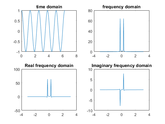
Discrete Fourier transform of a sinusoidal signal
17.4.1. Periodicity in the Frequency Domain
Sampling a continuous signal is equivalent to multiplying the signal with
the comb function with period of . Normally, when we think of
filtering, we do convolution in the time domain, which corresponds to
multiplication in the frequency domain. In this case, multiplication was
done in the time domain, so convolution is done in the frequency domain.
Referring to Common Fourier Transform Pairs, we see that the comb function is periodic
at every  Hz (cycles/second). Thus, discrete signals are
periodic in the frequency domain every coefficients.
Hz (cycles/second). Thus, discrete signals are
periodic in the frequency domain every coefficients.
Each sample point of the comb function is like an impulse signal, which
has a flat frequency response. So in the frequency domain, the shape of
the frequency response for the continuous and discrete signal are the
same over Hz or samples. The
DFT result is just
repeated every samples.
The periodic property can also be seen be in the equation for the DFT.
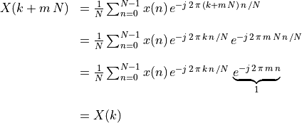
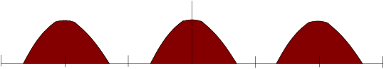
Discrete signals in frequency domain are periodic
17.4.2. Aliasing and Nyquist Theorem
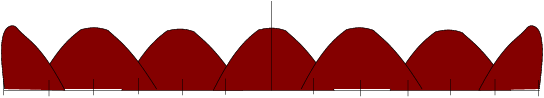
Since discrete signals and images are periodic in the frequency domain, if
the frequency response extends beyond  from zero, then they
will overlap with adjacent frequency response producing distortion know as
aliasing. Aliasing can occur either because of image or signal
processing, such as down sampling (resizing) an image, or because of not
sufficiently low pass filtering the signal before sampling.
from zero, then they
will overlap with adjacent frequency response producing distortion know as
aliasing. Aliasing can occur either because of image or signal
processing, such as down sampling (resizing) an image, or because of not
sufficiently low pass filtering the signal before sampling.
The Nyquist sampling theorem states that signals must be sampled at least twice the highest frequency component of the signal.
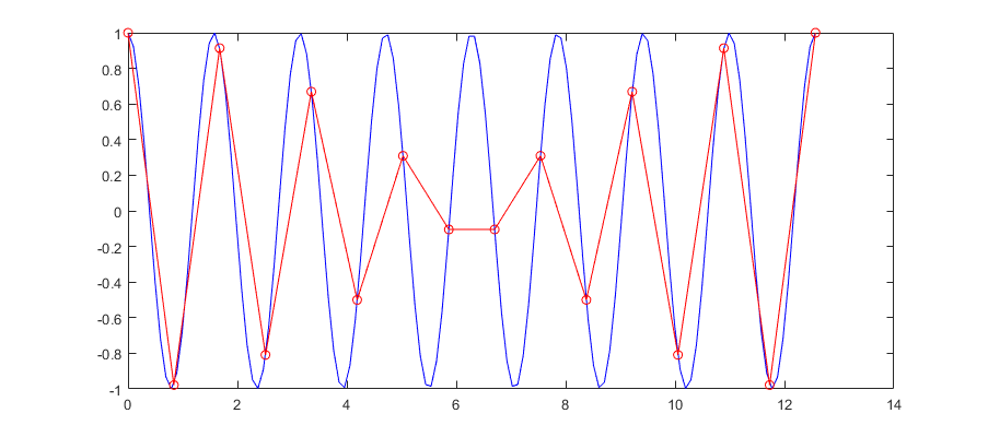
The red line tries to sample the blue line, but shows aliasing because it is undersampled, violating the Nyquist theorem.
Aliasing in the frequency domain
This video by Peter Corke demonstrates aliasing and how it occurs in the spatial domain.