17.3. Continuous 1D Fourier Transform
The Fourier Series previously considered is intended for use with periodic signals. More general signals may exhibit some locally periodic components, but are not, in general, periodic. The Fourier transform and the inverse Fourier transform allow for the conversion of any signal to the frequency domain and back again to either the time or spatial domain.
We consider one dimensional signals only as steps towards the 2-D Fourier transform of images. One dimensional continuous and discrete signals provide simpler cases for learning some of the important properties of frequency domain data.
-
Fourier Transform 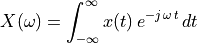
Where
 is a continuous frequency in radians/sec.
-
Inverse Fourier Transform 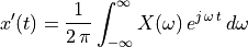
-
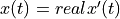
Properties  is continuous and may be complex.
 is complex and continuous.
 is complex, but if was real, then
 .
.- Although it is a bit hard to think about negative frequencies, they
are a mathematical necessity. This is because of the cyclical nature
of the complex exponential. The values of the complex exponential
over the range
 are the same as for the
equivalent range
are the same as for the
equivalent range  .
.
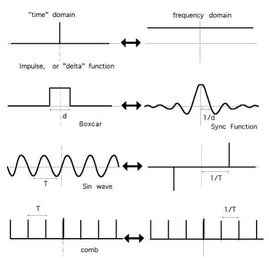
17.3.1. Common Fourier Transform Pairs
Below are some common frequency and time domain pairs. These results will be useful to us for explaining other properties later.