17.2. The Complex Exponential Basis Function
Note
Recall that a complex number is one containing a real component and an
imaginary component. Imaginary numbers are multiplied by the imaginary
number,  .
.

Mathematicians usually use the variable  as the imaginary
number. Engineers, however, prefer to use the variable
as the imaginary
number. Engineers, however, prefer to use the variable  .
Equations involving complex numbers often involve variables representing
voltage and current in a circuit. In electrical circuits, is
always current, so to avoid confusion, the variable is used
for the imaginary number.
.
Equations involving complex numbers often involve variables representing
voltage and current in a circuit. In electrical circuits, is
always current, so to avoid confusion, the variable is used
for the imaginary number.
As we saw, the Fourier Series generates a periodic signal as a sum of weighted sinusoidal signals. The Fourier transform extends the Fourier series to convert any continuously integrable signals into the frequency domain. The coefficients in the frequency domain are complex numbers to quantify both the magnitude and phase of the spectrum over a range of frequencies. In both the Fourier transform (FT) and inverse Fourier transform (IFT), we use the complex exponential basis function for the sinusoidal foundation of the transforms. The coefficients are calculated as a sum of products between the signal and the set of complex, sinusoidal basis functions. The complex exponential basis function is defined by what is called Euler’s formula.
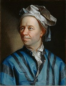
Leonhard Euler (1707 - 1783)

Euler What?!
Most people find Euler’s formula quite puzzling when they first see it. We
know that is the imaginary number  , but what is
 and what does it have to do with the
  and
and
 ?
?
17.2.1. The number 
Like the number  , the number
  is a
constant irrational number with a significant influence on the mathematics
of how things work. The value of is defined in terms of a limit.
is a
constant irrational number with a significant influence on the mathematics
of how things work. The value of is defined in terms of a limit.
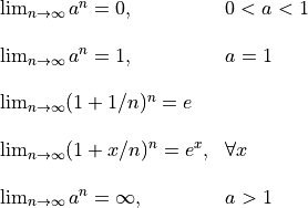
Here are the limits of exponentials that we already know about and
also the limits defining the number and also  .
.
The function has a couple properties that make it special.
- is the only known function that the derivative of the function
is itself. This causes to be in the solution to
many differential equation problems. Some examples where you will find
are: the voltage on a capacitor as a function of time, the
decay of radioactivity of the nucleus of an unstable atom, and the
probability density function of a Gaussian random variable.
- Euler’s formula, which we will tackle next.
17.2.2. Derivation of Euler’s Formula
We can see how  relates to the
  and
and
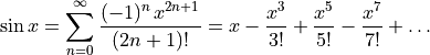
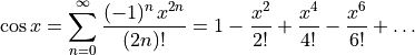
 functions by looking at the MacLaurin series for these
functions. A MacLaurin series is a Taylor series expansion about at the
point zero.
functions by looking at the MacLaurin series for these
functions. A MacLaurin series is a Taylor series expansion about at the
point zero.
If you are like I was as an undergraduate, Taylor and MacLaurin series expansions where among my least favorite parts of calculus class. However, they have two important virtues.
- They are useful for numeric calculations. Many years ago, before the days of computers and calculators, tables were used to find the value of many math functions. The people with the jobs of computing these tables often used Taylor and MacLaurin series to calculate the values in the tables. Calculators and computers might also use these series for internally calculating the values of some functions.
- There are some mathematical properties of functions that can only be observed by considering these series. This is the case with Euler’s formula for complex exponentials.
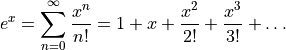
The needed MacLaurin series are:
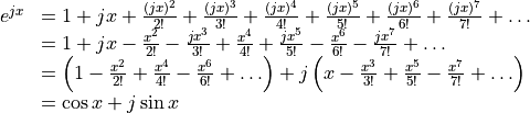
Now replace  in the equations for with
  .
Remember that
.
Remember that  .
.
17.2.3. Numerical Proof
Okay, if the derivation from the MacLaurin series didn’t convince you, we can try some numerical analysis to show that complex exponentials can actually produce complex, sinusoidal functions?
We can use MATLAB and the definition of from a limit and
verify if Euler knew what he was talking about or not. In the following
MATLAB script, we just assign  to be a fairly large number.
Since the definition uses a limit as goes to infinity, the
results become more accurate when larger value for are used.
to be a fairly large number.
Since the definition uses a limit as goes to infinity, the
results become more accurate when larger value for are used.
% let n = some big number
n = 100000;
z = linspace(0,2*pi); % test 100 numbers between 0 and 2*pi

% Now show that e^jz = cos(z) + j*sin(z)
% Begin with definition of value of e^z.
%    e^z = lim(n = infinity) (1 + z/n)^n
eulerValues = complex(1, z/n).^n;

% This should plot a unit circle, just like
% figure, plot( cos(z), sin(z));
figure, plot(real(eulerValues), imag(eulerValues));
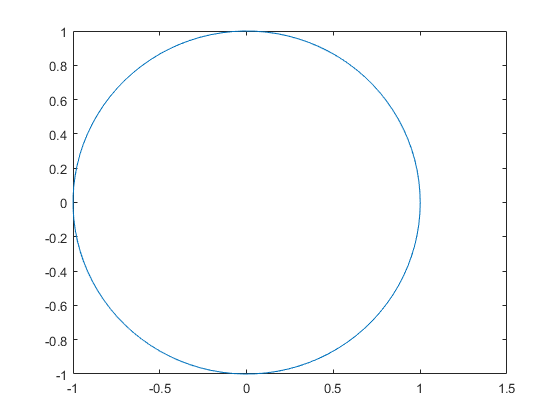
Points along a complex unit circle - Numerical proof of Euler’s formula
Note
One might reasonably suspect that MATLAB, being aware of Euler’s formula, cheated on calculating the complex exponential. That is, it probably converted the complex number to polar coordinates before doing the exponential calculation.
To complete the numerical proof, we can write a MATLAB function to do the complex exponential calculation by brute force. We will do this as a class activity and we will see the same result, which demonstrates the numerical validity of Euler’s formula.
17.2.4. But Why?
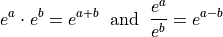
Representing the basis function as a complex exponential function is a more compact representation than the equivalent complex, sinusoidal expression. More importantly, the algebra rules for working with exponential functions of the same base simplifies the math for manipulating the basis functions. Namely …