17.1. Fourier Series
17.1.1. Jean Baptiste Joseph Fourier (1768-1830)

Crazy idea in 1807:
Any periodic function can be rewritten as a weighted sum of sines and cosines of different frequencies.
His idea was not accepted by most mathematicians of his day (Lagrange, Laplace, Poisson, … )
His work was not translated into English until 1878!
Today the Fourier Series is the primary tool for analysing signals, including images, in the frequency domain.
The Fourier Transform is the tool for converting signals from the time or spatial domains to the frequency domain.
17.1.2. Fourier Series of a Square Wave
As an example of a Fourier series, a square wave with a period of
 can be expressed with the following Fourier series.
Using MATLAB we can see that with just a few terms of the Fourier series, it begins to take the shape of a square wave.
>> theta = linspace(0,4*pi); % let theta be 2*pi*t/T. Show 2 cycles.
>> sq1 = sin(theta);
>> sq2 = sin(3*theta)/3;
>> sq3 = sin(5*theta)/5;
>> sq4 = sin(7*theta)/7;
>> plot1 = 4/pi * sq1;
>> plot2 = 4/pi * (sq1 + sq2);
>> plot3 = 4/pi * (sq1 + sq2 + sq3);
>> plot4 = 4/pi * (sq1 + sq2 + sq3 + sq4);
>> figure;
>> subplot(2,2,1), plot(theta, plot1), title('one term');
>> subplot(2,2,2), plot(theta, plot2), title('two terms');
>> subplot(2,2,3), plot(theta, plot3), title('three terms');
>> subplot(2,2,4), plot(theta, plot4), title('four terms');
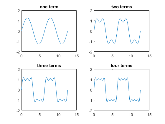
First Four Terms of the Fourier Series of a Square Wave
17.1.3. Adding Phase
In the square wave Fourier series, the phase of all of the sinusoidal terms are in phase with each other. Unfortunately, this is usually not the case. A more general expression of a Fourier series should incorporate phase as well as frequencies.
Let  and
and  each be magnitude and phase coefficients
of the Fourier series terms from a periodic signal
each be magnitude and phase coefficients
of the Fourier series terms from a periodic signal  with period
.
with period
.
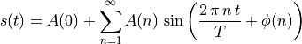
The above equation would be rather awkward to implement. Fortunately, we can express it with a more tractable equation. We will use complex numbers to do so. We will see next that the complex exponential yields a more eloquent expression for converting both periodic and non-periodic signals to the frequency domain using the Fourier transform and the inverse Fourier transform to convert the signal back to the time domain.
Note
To ease our introduction to images in the frequency domain, we will progress in steps.
First we will consider the complex exponential basis function of the Fourier transform. Many text books asks the reader to take the complex exponential as a given with out explaining it. I find this confusing.
Then we will consider the Fourier transform and its inverse for the following types of signals.
- One dimensional analog signals.
- One dimensional discrete or sampled signals.
- 2-D discrete images.