10.2. Perspective Projection Model
The previous diagram (Thin Lens Camera Model) accurately depicts the geometry of a camera. However, it does not yield a convenient mathematical model to relate points in the real world to points in the image.
The perspective projection model allows us relate object locations in the real world to the corresponding pixel locations in the image.
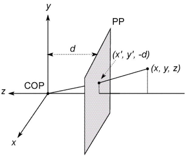
Perspective Projection Camera Model. In this diagram, the  and
and
 are as we normally view 2-D plots, so by the right hand rule the
 values of objects in the world are negative. Not everyone does it
this way.
values of objects in the world are negative. Not everyone does it
this way.
With the origin of the image coordinate system,  , in the
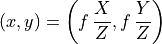
center of the image, the perspective projection equation relates the
world locations to image locations.
, in the
center of the image, the perspective projection equation relates the
world locations to image locations.
Notice that given a location in the world, it is possible to determine the image location, but not the reverse. An image point defines a ray, which might intersect an object in the world at any distance away. Some knowledge of the geometry of the world is required to determine world locations from an image.
For film cameras, it is appropriate to think of  in units of linear
distance; but for digital cameras, pixels is a more convenient unit for
. When is given in linear units (usually mm) for a
digital camera, the linear size of the distance between pixels,
in units of linear
distance; but for digital cameras, pixels is a more convenient unit for
. When is given in linear units (usually mm) for a
digital camera, the linear size of the distance between pixels,
 , must also be used. The unit of is usually
mm/pixel. Divide the focal length (mm) by
(mm/pixel) to get the focal length in pixels.
, must also be used. The unit of is usually
mm/pixel. Divide the focal length (mm) by
(mm/pixel) to get the focal length in pixels.
Another observation from perspective projection is that as
(distance from the camera) increases, objects in the image get
smaller. Thus parallel lines that are not perpendicular to the optical axis
appear to come to a point at a long distance away.

Figure 11.4 from [RVC] shows that parallel railroad tracks appear to come to a point at a long distance away.
When objects are very far away, the  ,
,  , and can be
huge. If the camera is moved, those numbers hardly change. This explains why
the moon seems to follow you, why the north star (Polaris) is always north, and
why you can tell time from the sun regardless of where you are.
, and can be
huge. If the camera is moved, those numbers hardly change. This explains why
the moon seems to follow you, why the north star (Polaris) is always north, and
why you can tell time from the sun regardless of where you are.
10.2.1. When Z is Constant
In industrial robotics applications it is common to position the camera so
that is constant. For to be constant, the axis of the
camera must be perpendicular to a flat surface being photographed. Images
from a camera positioned over a conveyor belt carrying products can meet this
scenario, as can a picture taken directly in front of a building.
When is constant and known, the ratio of  in
the perspective projection equation is constant for the whole image, so
the size of objects can be measured from the distance (in pixels) between
two points on the image.
in
the perspective projection equation is constant for the whole image, so
the size of objects can be measured from the distance (in pixels) between
two points on the image.
The distance between two points in an image is:

Then, the distance between the points in the world can be computed.


Note: The most accurate results are obtained from points near the optical axis (center) of the image.
The ratio of the distances between points in the image and points in the world is also constant. Thus, if we know the distance between two points in the world, then the distance between two other points can be calculated from an image.

10.2.2. Projective Geometry
In the matrices used to relate points from an image to points in the physical world, we use homogeous coordinates, rather than Euclidean coordinates. In one sense, this may seem as just a convenience to allow matrix multiplication by adding another row to the matrices; but it is really more than that. Homogeneous coordinates are used in the geometry system known as projective geometry, which describes the relationship between the physical world and images taken by cameras.

Urbino, Italy, The ideal city, by Piero della Francesca (1415–1492)
Projective geometry is concerned with how the world appears to us; whereas, Euclidean geometry describes the actual dimensions of objects. The images that our eyes send to the brain are projective views. Then our brain translates the projective images to Euclidean space to give us our intuition about the dimensions of the objects that we see. Artists were the first to recognize the importance of projective geometry. Projective geometry has its origins in the early Italian Renaissance, particularly in the architectural drawings of Filippo Brunelleschi (1377–1446) and Leon Battista Alberti (1404–1472), who invented the method of perspective drawing. Italian fresco painter Piero della Francesca (1415–1492) described the mathematical model of projective geometry in his publication De Prospectiva Pingendi in 1478. Later, French mathematician Gérard Desargues (1591–1661) gave us more rigorous mathematical models and equations of projective geometry that we use today. Two other 17th century mathematicians that contributed to our knowledge of projective geometry were Blaise Pascal and Philippe de La Hire.
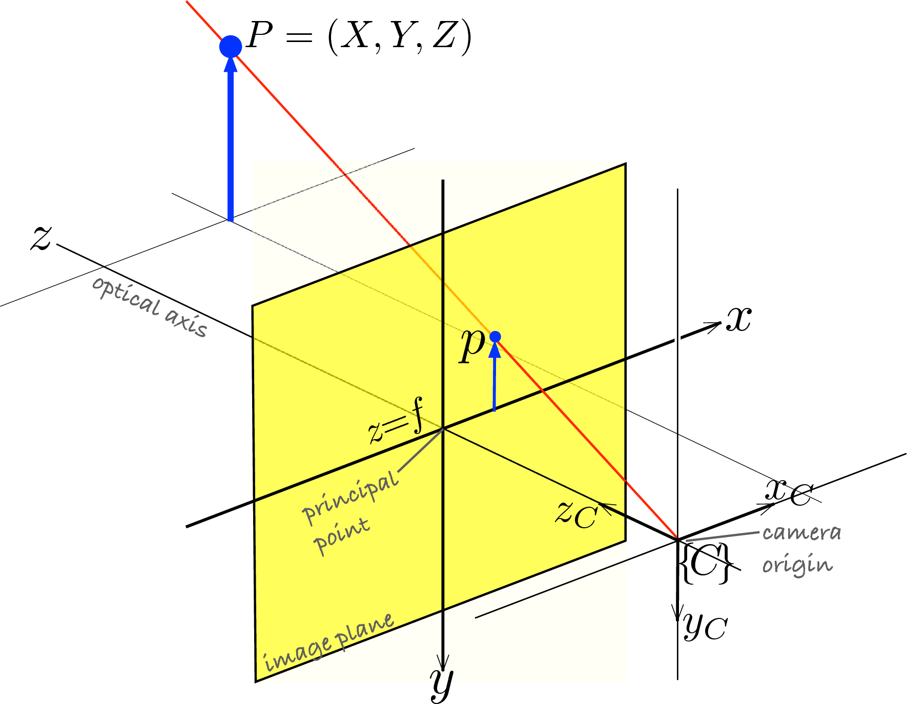
Figure 11.3 from [RVC]. This drawing illustrates the concept of projective
geometry as an artist should view a scene that they are drawing or painting.
Notice that in this diagram, the and axes point in the
same direction as  and
and  that we use with MATLAB. By the
right hand rule, the values of objects in the world are positive,
but the positive values are below the principal point.
that we use with MATLAB. By the
right hand rule, the values of objects in the world are positive,
but the positive values are below the principal point.
Here, we review a few math principles of projective geometry and homogeneous coordinates. Later, we will apply homogeneous coordinates to images.
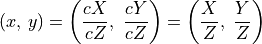
Consider a normalized projective system where, per the above diagram,
 , then any point
  passing through the image
(Euclidean) plane at point
passing through the image
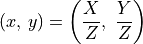
(Euclidean) plane at point  is on the same ray. Simply divide
 by to convert from homogeneous coordinates to
Euclidean coordinates.
by to convert from homogeneous coordinates to
Euclidean coordinates.
To convert a point in Euclidean coordinates to homogeneous coordinates, simply add an addition variable of value 1. Points along the same ray are scale invariant because any change is removed in the conversion back to Euclidean coordinates.
The 3-tuple homogeneous coordinate points are said to be in two dimensional
projective space ( ), that is, they
correspond to points on a plane in Euclidean space
(
), that is, they
correspond to points on a plane in Euclidean space
( ).
).
Representing points and lines in homogeneous coordinates allows us to take advantage of some convenient properties.
Consider two homogeneous points,  and
and
 , then the line between the points is the
cross product of the points.
, then the line between the points is the
cross product of the points.
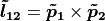
A line in homogeneous coordinates is also a 3-tuple. The point where two lines intersect is also found by a cross product.

See also
Data Analysis study guide for notes on cross products.
10.2.3. Camera Matrix
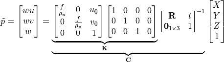
Here we discuss how to describe the perspective projection camera model with matrices such that the model is more useful as a software model.
In homogeneous coordinates, a point in the physical world is ideally projected onto an image with the following matrix multiplication.
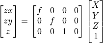
Note
The Euclidean coordinates of a point relative to the
principal point is  .
.
This model is appropriate for a continuous (film) image plane. But for
digital cameras, we have to divide the image plane into a grid of light
sensors (pixels). The dimension of each pixel in this grid is
 wide and
  high. The pixels on typical digital
camera are usually square, about 10 microns (
high. The pixels on typical digital
camera are usually square, about 10 microns ( meters) on each
side.
meters) on each
side.
In MATLAB, the origin is in the upper, left corner of the image, so we can translate the image to shift the origin from the principal point.
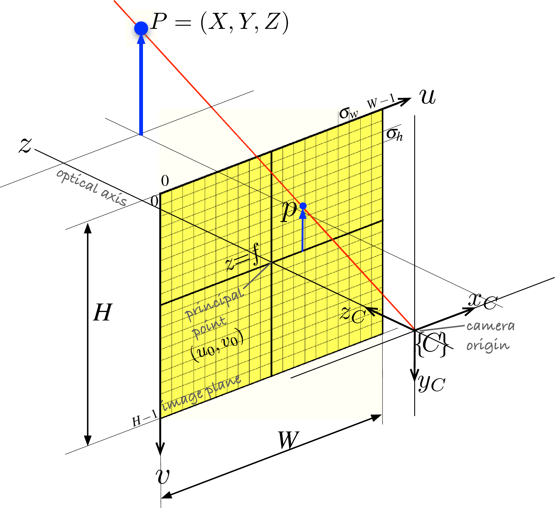
Figure 11.6 from [RVC]. This drawing is of the perspective projection camera model, but it also illustrates the concept of projective geometry.
To make the equations even more useful to machine vision applications, we can relate the position and orientation (pose) of the camera relative to a world coordinate frame.
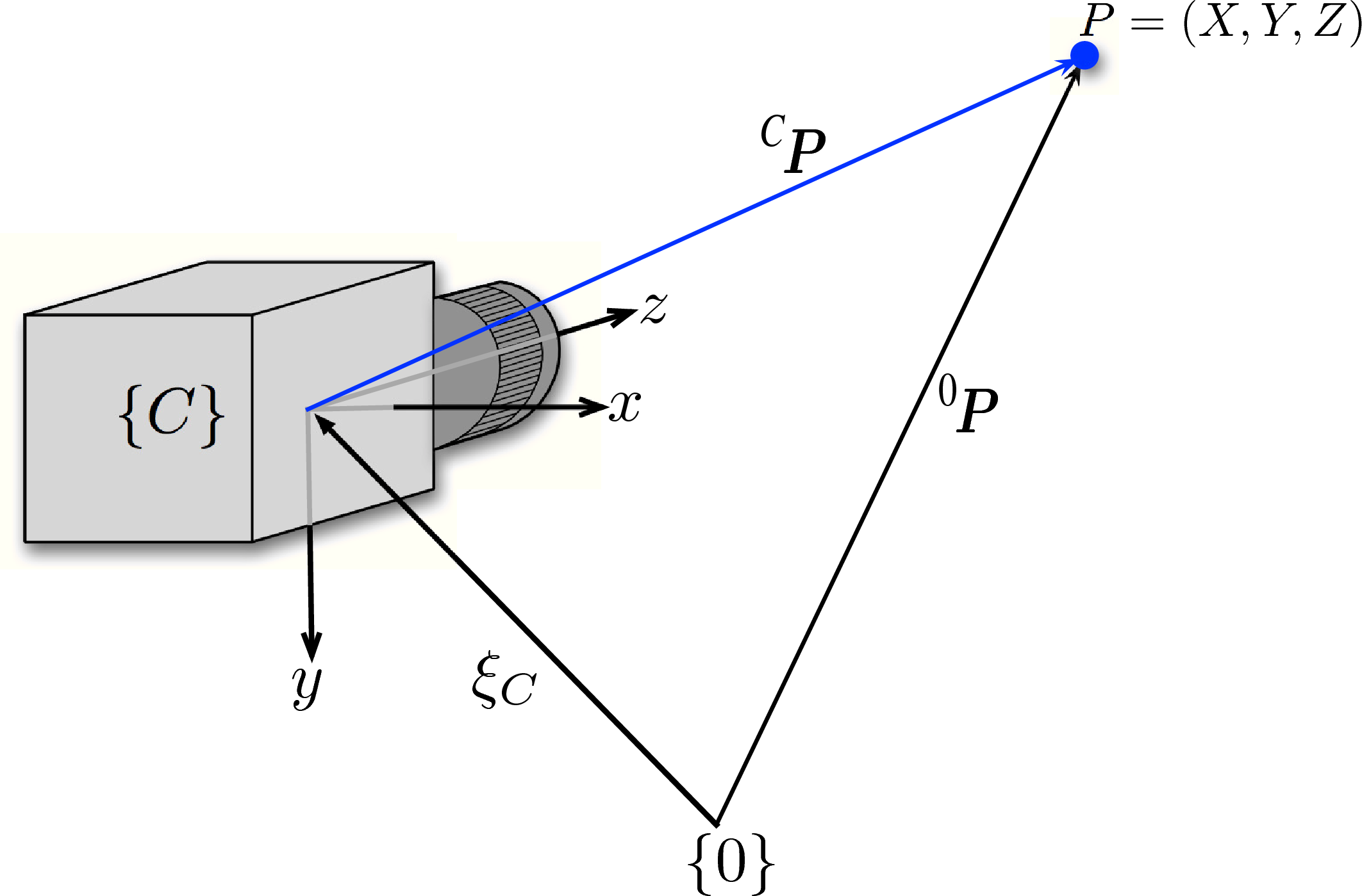
Figure 11.5 from [RVC]. The camera may be translated and rotated relative to a world coordinate frame.
Note
The  and
and  terms allow us to use the upper right
corner of the image as the origin. The coordinates of a point
terms allow us to use the upper right
corner of the image as the origin. The coordinates of a point  is again found by converting from homogeneos coordinates to Euclidean
coordinates,
is again found by converting from homogeneos coordinates to Euclidean
coordinates,  .
.
The product of the first two matrices is typically denoted by the symbol
 and we refer to these as the intrinsic parameters. All the
numbers in these two matrices are functions of the camera itself. It does not
matter where the camera is or where it is pointing, they’re only a function of
the camera. These numbers include the height and width of the pixels on the
image plane, the coordinates of the principal point, and the focal length of
the lens.
and we refer to these as the intrinsic parameters. All the
numbers in these two matrices are functions of the camera itself. It does not
matter where the camera is or where it is pointing, they’re only a function of
the camera. These numbers include the height and width of the pixels on the
image plane, the coordinates of the principal point, and the focal length of
the lens.
The third matrix describes the extrinsic parameters related to where the camera is but it does not say anything about the parameters of the camera.
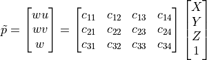
The product of these matrices is called the camera matrix,  .
.

The camera matrix can also be found from a calibration procedure, which may be needed if some parameters are not known or if the lens causes any distortion to the image.
Note
The value of  is often set to 1, in which case,
is said to be a normalized camera matrix.
is often set to 1, in which case,
is said to be a normalized camera matrix.
The MVTB has objects that model the projection of points onto an image plane of cameras with known parameters.
-
Example Given a camera matrix and point in the world as below, find where the point will be in an image.
>> C
C =
        512        -110           1         800
        512         512        -100        1600
          1           1           0           0
>> P
P =
    20
    30
    60

>> P_tilde = [P;1]  % homogeous coordinates
P_tilde =
    20
    30
    60
     1

>> p_tilde = C*P_tilde
p_tilde =
        7800
       21200
          50
>> p = p_tilde(1:2)/p_tilde(3) % Cartesian coordinates
p =
   156
   424
The image plane point is at
 .
.