10.3. Homography
When points in the world lie on a plane and we have some calibration location information about certain points, then we can use a technique called homography to find the locations of other points from an image. That is, we can find a geometric Transformation Matrix in homogeneous coordinates to map points from the image to their world coordinates on the plane.
The coordinate system for the world that we will use lies on the plane
so that every point that lies on this plane has a  value of zero.
We can show this in the Camera Matrix as:
value of zero.
We can show this in the Camera Matrix as:
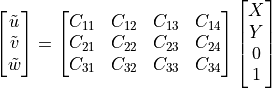
The multiples all of the elements in the third column
of our camera matrix. But because it is zero, we can effectively remove that
column from the matrix and we can remove that row from the world coordinate
vector.
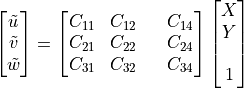
What we’re left with now is a 3-by-3 camera matrix for objects that are on a
plane. The inverse of the camera matrix is called a planar homography
( ) matrix that can find the coordinates of points on the plane
from the
) matrix that can find the coordinates of points on the plane
from the  locations in the image. We can estimate the homography
matrix if we have four world points and the corresponding position of those
points in the image.
locations in the image. We can estimate the homography
matrix if we have four world points and the corresponding position of those
points in the image.
Note that the homography matrix gives us a geometric transformation between two planes. We will consider it here as a mapping from the image plane to a physical plane, but it could map between two image planes. The inverse of a homography provides the reverse mapping between the two planes.
We can apply homographies in two ways. First we can do perspective rectification, which is a warping of the image to the coordinates of the physical world, much like the Geometric Operations that we considered before. The resulting image looks as if the picture was taken with the camera held orthogonal to the plane.
When we learn about finding objects in an image from their Image Features, we can also apply homography to find the location of specific objects from an image.
Look up the documentation of the following functions provided by the Machine Vision Toolbox:
- homography
- homwarp
- homtrans
Consider four points in an image making matrix  and the
corresponding points in the world in matrix
and the
corresponding points in the world in matrix  . The points in
might be calibration points and represents where
those calibration points were found in the image. With a homography matrix, we
can easily find the world location of other points found in the image.
. The points in
might be calibration points and represents where
those calibration points were found in the image. With a homography matrix, we
can easily find the world location of other points found in the image.
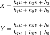
The homography mapping from to is in homogeneous
coordinates ( and
and  ). The
transformation is
). The
transformation is  . We might
hope to find using a similar linear algebra calculation as used
to solve a classic system of linear equations of the form
. We might
hope to find using a similar linear algebra calculation as used
to solve a classic system of linear equations of the form
 . However, this problem is more complex.
We have the following for each pair of corresponding points between image points and the world points on a plane.
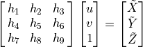
Additionally, the homogeneous coordinate requirement is that  and
and  . Letting
 , the equation for
  is combined with
equations for
is combined with
equations for  and
and  .
.
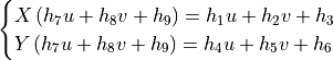
Then we have the following two equations for each pair of corresponding points.
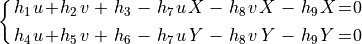
With  pair of corresponding points, which is the minimum, we have
eight equations of the form above. The coefficients of are put
into a column vector and the multipliers make an
pair of corresponding points, which is the minimum, we have
eight equations of the form above. The coefficients of are put
into a column vector and the multipliers make an  matrix of eight
rows (the rank of is 8).
matrix of eight
rows (the rank of is 8).
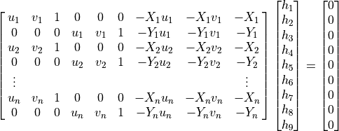
There are then two ways to solve the system of equations.
As shown above, the
matrix is  and the
 vector is
  ,
,  . So the null solution of gives the
values. A numerically stable way to solve for is to find the
singular value decomposition (SVD) factoring of (
. So the null solution of gives the
values. A numerically stable way to solve for is to find the
singular value decomposition (SVD) factoring of ([U,S,V] = svd(A)), and then the null solution is the last column of the matrix (
h = V(:, end)).Since the system of equations has eight degrees of freedom, the
 term can be set to 1 and the
  and
and  values moved to the
other side of the equal sign giving a
values moved to the
other side of the equal sign giving a  vector of 8 values.
Now we have a system of equations of the form
vector of 8 values.
Now we have a system of equations of the form  . But in case there are more than four pair of corresponding points,
the first 8
. But in case there are more than four pair of corresponding points,
the first 8  values are found from either using the pseudo-inverse
of (
values are found from either using the pseudo-inverse
of (h = pinv(A)*b) or as follows.
To find directly from and
in Euclidean coordinates, the MVTB has an homography function. The
location of any points on the plane are then found with the homtrans
function from the corresponding points in the image.
>> P = [10 12 80 95; 120 450 130 500]
P =
    10    12    80    95
   120   450   130   500
>> Q = [10 10 90 90;10 500 10 500]
Q =
    10    10    90    90
    10   500    10   500

>> H = homography(P, Q)
maximum residual 1.589e-14
H =
    1.3672   -0.0029   -2.5446
   -0.2518    1.8681 -210.8748
    0.0014    0.0005    1.0000

>> Q1 = homtrans(H, P)  % Test if the homography applied to P gives Q.
Q1 =
    10    10    90    90
    10   500    10   500
% Same result from: h2e( H * e2h(P) )
% e2h - Euclidean to homogeneous, h2e - homogeneous to Euclidean
Take a picture from the side of or below an object with points that lie on a
plane. Find the homography matrix mapping points from the image to world
coordinates. Use the homwarp function to transform the image with
perspective rectification.
Here is example of perspective rectification.
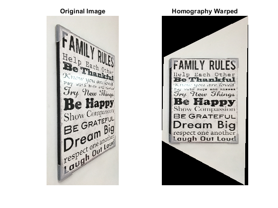
Homography image warp for perspective rectification