8. Geometric Operations
Reading Assignment
Please read section 12.7 of [RVC]; then read chapter 7 of [PIVP]; finally read section 14.2.4 of [RVC].
This chapter covers moving, removing, and duplication of pixels within an image.
8.1. Rotating a Pixel
Rotation is a very important topic to both machine vision and robotics. Pixels in an image might be rotated to align objects with a model.
Here, we only consider rotating points about the origin. Rotation about other points is an extension of rotating about the origin.
Point  is rotated by an angle
  about the
origin to point
about the
origin to point  .
.
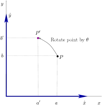
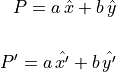
To facilitate the discussion, the point  is defined in terms of
unit vectors
is defined in terms of
unit vectors  and
and  . The new
location,
. The new
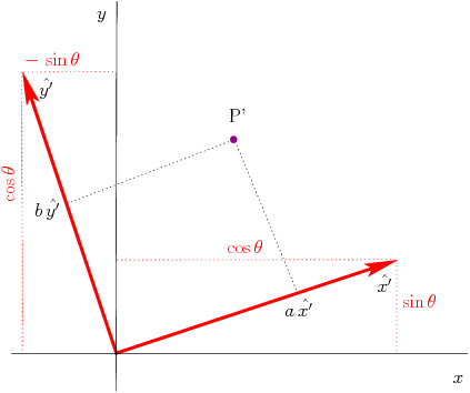
location,  is then defined by unit vectors
  and
and
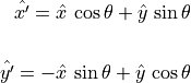
 formed by rotating
  and
and  by
the angle .
by
the angle .

Expressed in matrix notation:
![\begin{array}{ll}
P' &= \spalignmat{\hat{x}, \hat{y}}
\spalignmat[r]{\cos\theta, -\sin\theta;
\sin\theta, \cos\theta}
\spalignvector{a; b} \\ \\
&= \spalignmat{1, 0; 0, 1}
\spalignmat[r]{\cos\theta, -\sin\theta;
\sin\theta, \cos\theta}
\spalignvector{a; b} \\ \\
&= \spalignmat[r]{\cos\theta, -\sin\theta;
\sin\theta, \cos\theta}
\spalignvector{a; b}
\end{array}](../_images/math/f76d198baaf21754d8bbc22338e634213f7d2b61.png)
Thus, we have a 2-by-2 rotation matrix.
![R(\theta) = \spalignmat[r]{\cos\theta, -\sin\theta;
\sin\theta, \cos\theta}](../_images/math/2812e4fb3011bf7059afcb5a64e5921638ed8dbe.png)
The rotation matrix has the following special properties.
- The sum of each column is one.
- The columns are orthogonal. The dot product of the columns is zero. It is called an orthonormal matrix.
- The columns define unit vectors for the rotated coordinate frame.
 .
.- The determinant,
 , thus it
is never singular.
, thus it
is never singular.
8.2. Transformation Matrix
Geometric translation is often added to the rotation matrix to make a matrix
that is called the transformation matrix in homogeneous coordinates. The
translation coordinates ( and
and  ) are added in a third
column. To make the resulting matrix square, an additional row is also
added.
) are added in a third
column. To make the resulting matrix square, an additional row is also
added.
![T(\theta, x_t, y_t) = \spalignmat[r]{\cos\theta, -\sin\theta, x_t;
\sin\theta, \cos\theta, y_t;
0, 0, 1}](../_images/math/1c6c6be562042ecec77fecefc2899c018930d626.png)
This transformation matrix may then used in the image warping algorithm to find a new location for each pixel. This is referred to as a forward mapping.
![\spalignvector{x', y', 1} = \spalignmat[r]
{\cos\theta, -\sin\theta, x_t;
\sin\theta, \cos\theta, y_t;
0, 0, 1}\, \spalignvector{u, v, 1}](../_images/math/202c6048f355ca6ae195ec50e05f60885b3fd978.png)
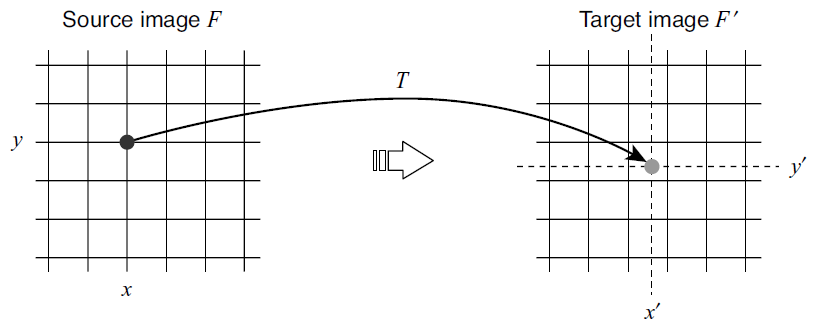
Figure 7.3 from [PIVP].
The location of each pixel from the source image is found in the target
image. This location  will likely be between actual pixel
locations in the target image. An interpolation algorithm could be used to
find the values for each pixel in the target image, but the nearest mapped
pixel is usually used with a forward mapping.
will likely be between actual pixel
locations in the target image. An interpolation algorithm could be used to
find the values for each pixel in the target image, but the nearest mapped
pixel is usually used with a forward mapping.
A more aesthetically pleasing result is achieved from a backward mapping image warping algorithm. In this approach, each pixel location from the target image is used to find the corresponding image location in the source image. This location will likely be between pixels in the source image, so an interpolation algorithm is used with the neighboring source pixels to determine the target pixel intensity.
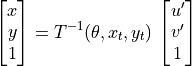

Figure 7.4 from [PIVP].
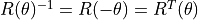
Note
The inverse of the homogeneous transformation matrix is not as simple to compute as it is for the rotation matrix. Whereas the inverse of a rotation matrix is found by simply taking the transpose of the matrix, the inverse of a homogeneous transformation matrix is a linear algebra matrix inverse.