9.2. The Classic SVD
We discuss the classic definition of the relationship between a matrix and it SVD factors in this section. The objective is to understand the relationship. We will consider the requirements and the difficulties associated with implementing the classic algorithm to compute the SVD.
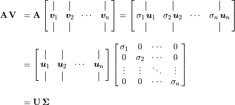
As with diagonalization factoring, a square matrix has  equations like
equation (9.1). Similarly, the vector equations can be
combined into a matrix equation. For a square, full rank matrix it looks as
follows.
equations like
equation (9.1). Similarly, the vector equations can be
combined into a matrix equation. For a square, full rank matrix it looks as
follows.
Note
This matrix equation is written as for a square matrix
( ). For rectangular matrices, the
  matrix has either rows or columns of zeros to accommodate the matrix
multiplication requirements.
matrix has either rows or columns of zeros to accommodate the matrix
multiplication requirements.
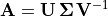
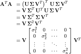
Then a factoring of  is
is
 , but a requirement of the
  vectors is that they
are orthogonal unit vectors such that
vectors is that they
are orthogonal unit vectors such that
 , so the SVD factoring of
is
, so the SVD factoring of
is
(9.2)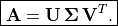
The factoring finds two orthogonal rotation matrices ( and
and
 ) and a diagonal stretching matrix
(). The size of each matrix is: :
) and a diagonal stretching matrix
(). The size of each matrix is: :
 , :
, :  ,
: , and
,
: , and  :
:
 .
.
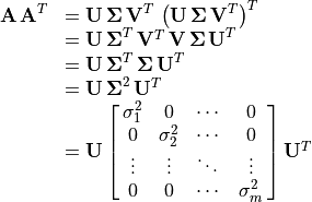
You may have correctly guessed that finding the SVD factors from
makes use of eigenvalues and eigenvectors. However, the
SVD factorization works with rectangular matrices as well as square
matrices, but eigenvalues and eigenvectors are only found for square
matrices. So a square matrix derived from the values of
is needed.
Consider matrices  and
and
 , which are always square, symmetric, and have
real, orthogonal eigenvectors. The size of
, which are always square, symmetric, and have
real, orthogonal eigenvectors. The size of  is , while the size of
 is . When we express
and with the SVD
factors, a pair of matrices reduce to the identity matrix and two
matrices combine into a diagonal matrix of squared
singular values.
is . When we express
and with the SVD
factors, a pair of matrices reduce to the identity matrix and two
matrices combine into a diagonal matrix of squared
singular values.
This factoring is the diagonalization of a symmetric matrix
(Diagonalization of a Symmetric Matrix). It follows that the matrix comes from
the eigenvectors of . Likewise, the
matrix is the square root of the diagonal eigenvalue
matrix of .
Similarly, the matrix is the eigenvector matrix of
.
Although comes from the eigenvectors of
, calculating as such is a poor
choice for square matrices and may not be necessary for rectangular
matrices.
9.2.1. Ordered Columns of the SVD
The columns of the sub-matrices are ordered according to the values of
the singular values ( ). The columns of and
are ordered to match the singular values.
). The columns of and
are ordered to match the singular values.
9.2.2. SVD of Square Matrices
If and are known, may
be found directly from equation (9.2). Since
 is orthogonal, its inverse is just .
The diagonal structure of makes its inverse the
diagonal matrix with the reciprocals of the
is orthogonal, its inverse is just .
The diagonal structure of makes its inverse the
diagonal matrix with the reciprocals of the  s on the
diagonal.
s on the
diagonal.
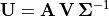
In MATLAB,  may be found with either the
pseudo-inverse,
may be found with either the
pseudo-inverse, pinv, function or the right-divide operator. For
full rank matrices the diag function could quickly find the inverse
of as (diag(1./diag(Sigma))), but care would be
needed to prevent a division by zero for singular matrices that have
singular values of zero.
U = A*V*pinv(Sigma);
  %  or
U = (A*V)/Sigma;
9.2.3. SVD of Rectangular Matrices
To satisfy the size requirements for multiplying the SVD factors, the
matrix contains rows of zeros for over-determined matrices
and columns of zeros for under-determined matrices. Figures
Fig. 9.1, and Fig. 9.2 show the related sizes of
the sub-matrices for over-determined and under-determined matrices.

Fig. 9.1 Shape of the SVD factors of an over-determined matrix.

Fig. 9.2 Shape of the SVD factors of an under-determined matrix.
9.2.4. The Economy SVD
Note that in the multiplication of the factors to yield the original
matrix,  columns of for an over-determined
matrix and
columns of for an over-determined
matrix and  rows of for an
under-determined matrix are multiplied by zeros from
. They are not needed to recover from
its factors. Many applications of the SVD do not require the unused
columns of or the unused rows of . So
the economy SVD is often used instead of the full SVD. The economy SVD
removes the unused elements.
rows of for an
under-determined matrix are multiplied by zeros from
. They are not needed to recover from
its factors. Many applications of the SVD do not require the unused
columns of or the unused rows of . So
the economy SVD is often used instead of the full SVD. The economy SVD
removes the unused elements.
Figure Fig. 9.3 shows the related sizes of the economy
sub-matrices for over-determined matrices. The primary difference to be
aware of when applying the economy SVD is a degradation of the unitary
properties of and  . For an over-determined
matrix
. For an over-determined
matrix  , but
, but
 .
Similarly, for an under-determined matrix
.
Similarly, for an under-determined matrix
 , but
, but
 .
.

Fig. 9.3 Shape of the economy SVD factors of an over-determined matrix.
We will resume the discussion of the economy SVD in Projection and the Economy SVD in the context of vector projections.
9.2.5. Implementation Difficulties
Finding the SVD using the classic algorithm is problematic.
A difficulty arising from the rows or columns of zeros in
and
is fraught with problems. If the eigenvectors of
for the factoring to be correct. It is best to do only one eigenvector calculation.
Some applications may have large
Small singular values of
for
for
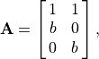
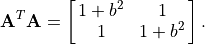
Golub and Reinsch [GOLUB70] offer a simple experiment to observe the lack of accuracy. Of course, the error that we see now with double precision floating point arithmetic is less than they would have observed using 1970 computers. Consider the matrix
then
The singular values are:
, and
. As the
variable is reduced from 0.01 by powers of 10 to
, then with the classic SVD algorithm small errors in
are returned from the beginning. The errors grow as
, the error is complete and
.
The difficulties associated with finding the SVD using the classic approach motivates the search for alternative algorithms, which are explored in Calculating the SVD with Unitary Transformations.
To complete the discussion of the classic SVD, econSVD
is a simple function that uses the classic algorithm to find the SVD
of a square matrix and the economy SVD of a rectangular matrix. The code
shown here is not how the SVD should be computed, but it reinforces the
relationship between a matrix and its SVD factors.
function [U, S, V] = econSVD(A)
% ECONSVD - an implementation of Singular Value Decomposition (SVD)
%           using the classic algorithm.
%           It finds the full SVD when A is square and the economy
%           SVD when A is rectangular.
% [U,S,V] = econSVD(A) ==> A = U*S*V'
%
% This function is for educational purposes only.

% Use the smaller of A'*A or A*A' for eig calculation.
    [m, n] = size(A);
    if m < n             % under-determined
        [U, S] = order_eigs(A*A');
        V = (A'*U)/S;
    else                 % square or over-determined
        [V, S] = order_eigs(A'*A);
        U = (A*V)/S;
    end
end

function [X, S] = order_eigs(B)
% helper function, B is either A'*A or A*A'
    [X2, S2] = eig(B);
    [S2, order] = sort(diag(S2), 'descend');
    X = X2(:, order);
    % There are no negative eigenvalues but we still need abs()
    % in the next line just because a 0 can be -0, giving an undesired
    % complex result.
    S = diag(sqrt(abs(S2)));
end
