11.2. Data Interpolation

Data interpolation algorithms are used to fill in the unknown data points between data points that are known.

11.2.1. One-Dimensional Interpolation

MATLAB has two functions that interpolate between one-dimensional data samples to estimate unknown points. The difference between the two functions relates only to the purpose for calling them. The fillmissing function is used when values that should be in the data are missing—often replaced with the NaN symbol. The interp1 function adds data points not contained in the data. We used fillmissing in Dealing with Missing Data when data imported into MATLAB had some missing values, and we will use interp1 in the examples in this section. We call interp1 with vectors for the given \(x\) and \(y\) data values (x1, y1), along with a longer vector of \(x\) values (x2) where we want to find corresponding interpolated \(y\) values. An optional fourth argument is a string listing the interpolation algorithm.

y2 = interp1(x1, y1, x2, <algorithm>)

Several interpolation algorithms are available. Five commonly used algorithms are:

’nearest’ n̄earest-neighbor interpolation

’linear’ linear interpolation, default

’pchip’ piecewise cubic Hermite interpolation

’makima’ modified Akima cubic Hermite interpolation

’spline’ cubic spline interpolation

MATLAB also has functions that directly invoke the data interpolation algorithms rather than invoking them via fillmissing or interp1. These functions include pchip, spline, and makima.

The default interpolation algorithm is ’linear’, which does not usually provide smooth transitions between points but is good when the given data changes slowly between sample points. The methods ’pchip’, ’makima’, and ’spline’ yield good results. The ’spline’ method requires the most computation because it uses a matrix computation for each point to determine polynomial coefficients that match the given data and maintain constant first and second order derivatives at each data point added. However, the ’spline’ method may overshoot data points, causing an oscillation. The results from the ’pchip’ and ’makima’ algorithms are similar. They maintain consistent first-order but not consistent second-order derivatives at each point. They avoid overshoots and accurately connect the flat regions. Another advantage of the ’pchip’ and ’makima’ algorithms is that if the given data points are either monotonically increasing or decreasing, so will the interpolated data points [HIGHAM17]. The ’spline’ interpolation may not always maintain data monotonicity because of oscillations. Since ’pchip’ and ’makima’ have similar results, only the ’pchip’ interpolation is used in the following comparison code and plots in figure Fig. 11.7.

f = @(x) 1 + x.^2 - x.^3 + 20*sin(x);
x1 = (-3:1.5:3)';  % Limited data points
y1 = f(x1);
x2 = (-3:0.5:3)';  % More data points
subplot(2,2,1)
plot(x1,y1,'o',x2,interp1(x1,y1,x2,'nearest'),'+:')
title('nearest'), subplot(2,2,2)
plot(x1,y1,'o',x2,interp1(x1,y1,x2,'linear'),'+:')
title('Linear'), subplot(2,2,3)
plot(x1,y1,'o',x2,interp1(x1,y1,x2,'pchip'),'+:')
title('pchip'), subplot(2,2,4)
plot(x1,y1,'o',x2,interp1(x1,y1,x2,'spline'),'+:')
title('spline')

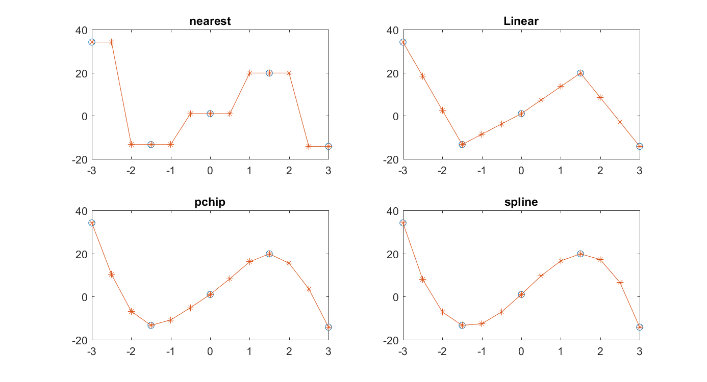
Fig. 11.7 Comparison of four data interpolation algorithms. The circles show the given data points, while the interpolated points are marked with plus signs.

The following example illustrates the difference between ’pchip’ and ’spline’ interpolation results. As figure Fig. 11.8 shows, the ’pchip’ result may not be as smooth, but the monotonicity of the data is preserved.

x = -3:3;
y = [-1 -1 -1 0 1 1 1];
t = -3:.01:3;
hold on
plot(x, y, 'o')
plot(t, interp1(x, y, t, 'pchip'), 'g')
plot(t, interp1(x, y, t, 'spline'), '-.r')
legend('data', 'pchip', 'spline', 'Location', 'NorthWest')
hold off

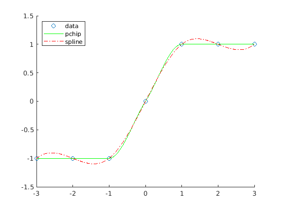
Fig. 11.8 Comparison of ’pchip’ and ’spline’ data interpolation

11.2.2. Two-Dimensional Interpolation

The two-dimensional interpolation functions griddata and interp2 follow in the same pattern as the one-dimensional functions. The inputs are matrices of grid points, such as returned from meshgrid, which we used in 3-D Plots to make surface plots. The distinction between griddata and interp2 is that interp2 requires that the grid data be monotonically increasing from meshgrid, while griddata does not have that requirement. The available interpolation methods are ’linear’, ’nearest’, ’cubic’, ’makima’, or ’spline’ with the default method again being ’linear’. In the following example, we will use the default interpolation. The appearance of the surface plot in figure Fig. 11.9 is indistinguishable from a surface plot where all of the points come from an equation rather than having some interpolated points.

>> [X, Y] = meshgrid(linspace(-10, 10, 20));
>> T = X.^2 + Y.^2;
>> Z = (Y-X).*exp(-0.12*T);
>> [Xi, Yi] = meshgrid(linspace(-10, 10, 40));
>> Zi = interp2(X, Y, Z, Xi, Yi);
>> surf(Xi, Yi, Zi)

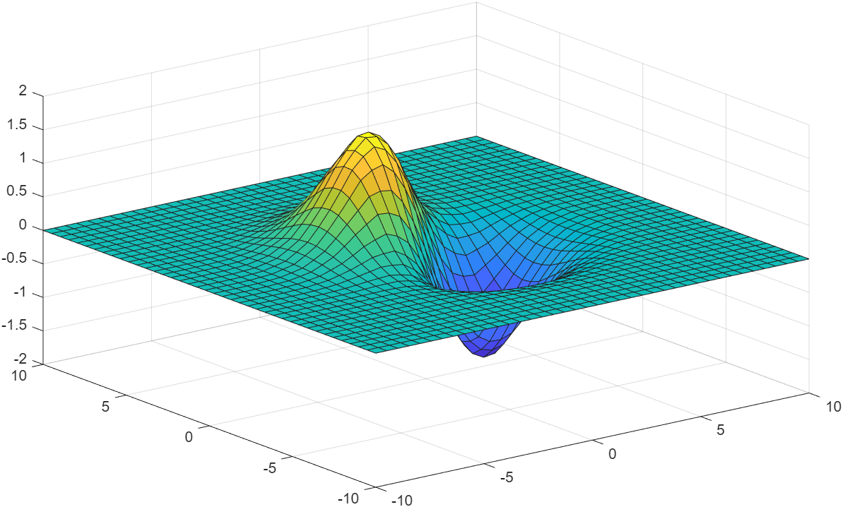
Fig. 11.9 A surface plot where half of the data points are found from linear interpolation.