11.5. Numerical Differential Equations

An ordinary differential equation (ODE) is an equation of the form

\[y'(t) = \frac{dy}{dt} = f(t, y), \text{ with } y(t_0) = y_0.\]

We are given the rate of change, the derivative of \(y(t)\), from which we solve for \(y(t)\). Because we are also given the initial value \(y(t_0) = y_0\), this class of ODE problems is called an initial value problem (IVP). We will consider cases of the function \(y(t)\) representing a single equation and a system of equations.

Differential equations are important to engineers and scientists because they describe changes to the state of dynamic systems. These dynamic systems include moving objects, wires carrying fluctuating electrical current, fluid reservoirs with measurable pressure, temperature, and volume, or anything where the system’s state can be quantified numerically.

Numerical methods are especially needed to solve higher-order and nonlinear ODEs. As is the case with integration, our ability to properly evaluate some ODEs using analytic methods are less than satisfying [STRANG14]. So numerical methods for solving ODEs are important tools in the engineer’s computational toolbox.

This is our third encounter with ODEs. In Throwing a Ball Up, we used MATLAB’s Symbolic Math Toolbox to find the algebraic equations from the differential equations associated with the effect of gravity on a ball thrown upwards. Then, in Systems of Linear ODEs we considered systems of first-order linear ODEs that may be solved analytically with eigenvalues and eigenvectors. Now, we will consider numerical methods to find and plot the solutions to ODEs. We will cover the basic algorithmic concepts of how numerical ODE solvers work and review the efficient suite of ODE solvers provided by MATLAB.

Recall the definition of a derivative:

\[\frac{dy}{dt} = \lim_{h \rightarrow 0} \frac{y(t + h) - y(t)}{h}.\]

For discrete samples of \(y\), the derivative becomes

\[y_k' = \frac{y_{k+1} - y_k}{h},\]

where \(h\) is the distance between sample points, \(h = t_{k+1} - t_k\). Rearranged to find \(y_{k+1}\) from the previous value, \(y_k\), and the slope of the function at \(t_k\), we have

(11.1)\[y_{k+1} = y_k + h\,y'_k.\]

Equation (11.1) is the basis for the simplest ODE solver, Euler’s method. However, we are limited on how small \(h\) can be due to concerns about excessive computation and round-off errors. So the accuracy of equation (11.1) is unacceptable for most applications.

Since differential equations are given in terms of an equation for the derivative of \(y\), \(y' = f(t, y)\), and the initial value, \(y_0\), the general discrete solution comes from the fundamental theorem of calculus, which applies the anti-derivative of a function to a definite integral.

(11.2)\[y_{k+1} = y_k + \int_{t_k}^{t_{k+1}} f(t, y) dt\]

Then the numerical approximation comes from the algorithm used to calculate the definite integral.

(11.3)\[I_k = \int_{t_k}^{t_{k+1}} f(t, y) dt\]

At each step, the ODE solver uses a straight line with a slope of \(I_k/h\) to advance from \(y_k\) to \(y_{k+1}\).

11.5.1. Euler’s Method

Euler’s method uses a Riemann integral to approximate equation (11.3) with constant height rectangular subintervals. [1] It is a reasonable solution if \(f(t, y)\) is constant or nearly constant. However, the results from Euler’s methods applied to most ODEs are not accurate enough for most applications unless the step size is small enough relative to the rate of change of the \(f(t, y)\) function.

\[\begin{split}\begin{aligned} \int_{t_k}^{t_{k+1}} f(t, y) dt \approx h\,f(t_k, y_k) \\ y_{k+1} = y_k + h\,f(t_k, y_k) \end{aligned}\end{split}\]

Euler’s method is a perfect match if we let \(f(t, y) = a\), then

\[y_{k+1} = y_k + h\,a.\]

The \(y_k\) values may be expressed directly from the initial condition and the rate of change.

\[\begin{split}\left\{\begin{aligned} y_1 &= {y_0 + h\,a} \\ y_2 &= {y_1 + h\,a} {= y_0 + 2\,h\,a} \\ &\vdots \\ y_k &= {y_0 + k\,h\,a} \end{aligned}\right.\end{split}\]

First, define a function or function handle for the derivative. It should take two arguments, \(t\) and \(y\). Although in many cases, the function only operates on one variable—usually the second, \(y\), variable. The function should accept and return vector variables.

\[\frac{dy(t)}{dt} = f(t, y)\]

The eulerODE function implements Euler’s method. The first three arguments passed to eulerODE are the same as those used with the MATLAB ODE solvers. The first argument to eulerODE is the derivative function. Next, specify a tspan argument, which is a row vector of the initial and final \(t\) values [2] ([t_0 t_final]). The third argument is the initial value of \(y\), \(y_0 = y(t_0)\). The final argument is \(n\), the number of values to find. The returned data from the ODE solvers are the \(t\) evaluation points and the \(y\) solution.

>> f = @(t, y) 5
>> [t, y] = eulerODE(f, [0 10], 5, 4)
t =
         0    3.3333    6.6667   10.0000
y =
    5.0000   21.6667   38.3333   55.0000

Figure Fig. 11.18 shows a plot comparing the relative accuracy of Euler’s method to other fixed step size algorithms.

function [t, y] = eulerODE(f, tspan, y0, n)
% EULERODE - ODE solver using Euler's method.
%
%   f - vectorized derivative function, y' = f(t, y)
%   tspan - row vector [t0 tf] for initial and final time
%   y0 - initial value of y
%   n - number of y values to find
    h = (tspan(2) - tspan(1))/(n-1);
    t = linspace(tspan(1), tspan(2), n);
    y = zeros(1, n); y(1) = y0;
    for k = 1:n-1
        y(k+1) = y(k) + h*f(t(k), y(k));
    end

11.5.2. Heun’s Method

Heun’s method uses trapezoid rule integration to approximate equation (11.3).

(11.4)\[y_{k+1} = y_k + \frac{h}{2}\left[f(t_k, y_k) + f(t_{k+1}, y_{k+1})\right]\]

However, equation (11.4) makes use of \(y_{k+1}\), which is not yet know. So Euler’s method is first used to make an initial estimate (\(\tilde{y}_{k+1}\)). Because the algorithm makes an initial prediction of \(\tilde{y}_{k+1}\) and then updates the estimate with a later equation. Heun’s method belongs to a class of algorithms called predictor–corrector methods.

\[\tilde{y}_{k+1} = y_k + h\,f(t_k, y_k)\]

The complete Heun method equation is given by equation (11.5).

(11.5)\[y_{k+1} = y_k + \frac{h}{2}\left[f(t_k, y_k) + f(t_{k+1}, (y_k + h\,f(t_k, y_k)))\right]\]

The heunODE function is called with the same arguments as the eulerODE function.

function [t, y] = heunODE(f, tspan, y0, n)
% HEUNODE - ODE solver using Heun's method.
%
%   f - vectorized derivative function, y' = f(t, y)
%   tspan - row vector [t0 tf] for initial and final time
%   y0 - initial value of y
%   n - number of y values to find
    h = (tspan(2) - tspan(1))/(n-1);
    t = linspace(tspan(1), tspan(2), n);
    y = zeros(1, n); y(1) = y0;
    for k = 1:n-1
        fk = f(t(k), y(k)); yk1 = y(k) + h*fk;
        y(k+1) = y(k) + (h/2)*(fk + f(t(k+1), yk1));
    end

11.5.3. Runge-Kutta Method

The Runge-Kutta method uses Simpson’s rule integration to approximate equation (11.3). Several algorithms are considered to be part of the Runge-Kutta family of algorithms. The so-called classic algorithm used here is an order–4 algorithm with a comparatively simple expression. Runge-Kutta algorithms are the most accurate of the fixed-step size algorithms. They are only surpassed by adaptive step size algorithms, which typically use Runge-Kutta equations.

Runge-Kutta estimates are weighted sums of coefficients calculated from evaluations of \(f(t, y)\) (the derivative function). The equation’s latter coefficients use previous coefficients, so the coefficients at each evaluation point are calculated sequentially before the solution value can be determined.

\[\begin{split}\begin{array}{rl} &s_1 = f(t_k, y_k) \\ \hfill \\ &s_2 = f(t_k + \frac{h}{2}, y_k + \frac{h}{2}\,s_1) \\ \hfill \\ &s_3 = f(t_k + \frac{h}{2}, y_k + \frac{h}{2}\,s_2) \\ \hfill \\ &s_4 = f(t_k + h, y_k + h\,s_3) \\ \hfill \\ &y_{k + 1} = y_k + \frac{h}{6}\, \left( s_1 + 2s_2 + 2s_3 + s_4 \right) \end{array}\end{split}\]

The rk4ODE function is called with the same arguments as the eulerODE and heunODE functions.

function [t, y] = rk4ODE(f, tspan, y0, n)
% RK4ODE - ODE solver using the classic Runge-Kutta method.
%
%   f - vectorized derivative function, y' = f(t, y)
%   tspan - row vector [t0 tf] for initial and final time
%   y0 - initial value of y
%   n - number of y values to find
    h = (tspan(2) - tspan(1))/(n - 1);
    t = linspace(tspan(1), tspan(2), n);
    y = zeros(1, n); y(1) = y0;
    for k = 1:n-1
        s1 = f(t(k), y(k));
        s2 = f(t(k)+h/2, y(k)+s1*h/2);
        s3 = f(t(k)+h/2, y(k)+s2*h/2);
        s4 = f(t(k+1), y(k)+s3*h/2);
        y(k+1) = y(k) + (h/6)*(s1 + 2*s2 + 2*s3 + s4);
    end

11.5.4. Algorithm Comparison

We will use the well-known decaying exponential ODE to compare the three methods that use a fixed step size. We will also reference this simple ODE when considering stability constraints on the step size in Stability Constraints.

The ODE

\[y' = \frac{dy(t)}{dt} = -a\,y,\; \text{where}\; a > 0,\: \text{and}\: y(0) = c\]

has the solution \(y(t) = c\,e^{-at}\). For our comparison, \(a = 1\), and \(y(0) = 1\).

We can see in figure Fig. 11.18 that, as expected, the classic Runge-Kutta method performs the best, followed by Heun’s and Euler’s methods.

>> % Code for figure 11.18
>> f = @(t, y) -y;
>> [t, y_euler] = eulerODE(f, [0 4], 1, 8);
>> y_exact = exp(-t);
>> [t, y_heun] = heunODE(f, [0 4], 1, 8);
>> [t, y_rk4] = rk4ODE(f, [0 4], 1, 8);

Fig. 11.18 Comparison of fixed interval ODE solvers

Note

All algorithms shown in figure Fig. 11.18 perform well if \(h\) is significantly reduced. Notable differences can only be found using a larger step size.

11.5.5. Stability Constraints

An unstable algorithm execution gives fluctuating and wrong answers. A user without knowledge of the stability constraints could specify a step size for a fixed step size algorithm that is too large and get an unstable solution. The stability constraint is especially concerning with stiff systems [3] where one term in the solution may place a much higher constraint on the step size than other terms.

We return to the Euler method and an exponentially decaying ODE to find a stability constraint related to \(h\), the distance between consecutive evaluation points [SHEN15]. With \(y' = -a\,y\), where \(a > 0\), \(y(0) = 1\), the exact solution is \(y(t) = e^{-a\,t}\). A property of \(y(t)\) that needs to be preserved is that \(y(t) \to 0\) as \(t \to \infty\).

Referring to Euler’s Method, The forward Euler solution is \(y_{k+1} = y_k - h\,a\,y_k\), or \(y_{k+1} = (1 - ha)\,y_k\). By induction,

(11.6)\[y_k = (1 - ha)^k\,y_0.\]

A stability constraint on equation (11.6) is needed to ensure that the property of \(y_k \to 0\) as \(k \to \infty\) is preserved.

\[\begin{split}\begin{aligned} &\abs{1 - h\,a} < 1 \\ -1 &< (1 - h\,a) < 1 \\ -2 &< -h\,a < 0 \\ &h < \frac{2}{a} \end{aligned}\end{split}\]

In the following example \(2/a = 2/0.5 = 4\), but \(h = 5\) and the results are unstable [4].

>> fexp = @(t, y) -0.5*y;
>> [~, y_unstable] = eulerODE(fexp, [0 20], 1, 5)
y_unstable =
    1.0000   -1.5000    2.2500   -3.3750    5.0625

The stability constraint for Euler’s method is sufficient for other fixed-step size algorithms.

11.5.6. Implicit Backward Euler Method

The implicit backward Euler (IBE) method seeks to remove the stability constraint of fixed step size ODE solvers. To see how the IBE solver works, we will look at equation (11.2) from the perspective of finding \(y_k\) from the yet unknown \(y_{k+1}\). So the terms of equation (11.2) are reordered, and the integration limits are reversed.

(11.7)\[y_k = y_{k+1} + \int_{t_{k+1}}^{t_k} f(t, y) dt\]

Again, we will use the ODE \(y' = -a\,y\), where \(a > 0\), and \(y(0) = 1\). The exact solution is \(y(t) = e^{-a\,t}\). As before, we want to find any required stability constraints to ensure that \(y_k \to 0\) as \(k \to \infty\). We can solve the decaying exponential ODE problem numerically by applying Euler’s method to equation (11.7).

\[\begin{split}\begin{aligned} y_k &= y_{k+1} + h\,a\,y_{k+1} \\ y_k &= (1 + h\,a)\,y_{k+1} \\ y_{k+1} &= \frac{1}{1 + h\,a}\,y_k \end{aligned}\end{split}\]

(11.8)\[\begin{aligned} y_{k+1} &= \left(\frac{1}{1 + h\,a}\right)^k y_0 \end{aligned}\]

The constraint to ensure stability of equation (11.8) as \(k \to \infty\) requires that

\[\left\vert\frac{1}{1 + h\,a}\right\vert < 1,\]

which always holds because both \(h\) and \(a\) are positive numbers. So the implicit backward Euler method is unconditionally stable.

11.5.7. Adaptive Algorithms

Numerical ODE solvers need to use appropriate step sizes between evaluation steps to achieve high levels of accuracy while also quickly finding solutions across the evaluation interval. Adaptive ODE solvers reduce the step size, \(h\), where needed to meet the accuracy requirements. They also increase the step size to improve performance when the accuracy requirements can be satisfied with a larger step size.

One of two strategies can be used to determine the step size adjustments. Similar to adaptive numerical methods for computing integrals (Recursive Adaptive Integral), the solution from two half steps could be compared to the solution from a full step. Based on the comparison, the step size can be reduced, left the same, or increased. However, points of an ODE solution are found sequentially, so splitting a wide region into successively smaller intervals would be computationally slow. Instead, the current step size is used to find the next solution (\(y_{k+1}\)) using two algorithms, where one is regarded as more accurate. The guiding principle is that if the solutions computed by the two algorithms are close to the same, the step size is small enough or could even be increased. However, the step size should be reduced if the difference between the solutions is larger than a threshold. If the solutions differ significantly, then the current evaluations are recalculated with a smaller step size. The algorithm advances to the next evaluation step only when the solutions’ differences are less than a specified tolerance.

11.5.7.1. RKF45 Method

The Runge-Kutta-Fehlberg method (denoted as RKF45) uses fourth and fifth order Runge-Kutta ODE solvers to adjust the step size at each evaluation step. The fourth-order equation used is more complex than the one used by the fourth-order classic Runge-Kutta algorithm. However, the computed coefficients for the fourth-order equation are also used for the fifth-order equation, which only requires one additional coefficient. In the rkf45ODE function, the fourth-order solution values (RK4) are stored in the z array, and the fifth-order solution values (RKF45) are stored in the y array, which is returned from the function. The coefficients and solution values are calculated using the following equations. Note that the \(s_2\) coefficient is used to find later coefficients, but is not part of the fourth or fifth order solution equations.

There are variances in the literature on the implementation details of the RKF45 method. The rkf45ODE function is adapted from the description of the algorithm in the numerical methods text by Mathews and Fink [MATHEWS05].

\[\begin{split}\begin{aligned} &z_{k+1} = y_k + \frac{25}{216}s_1 + + \frac{1408}{2565}s_3 + \frac{2197}{4101}s_4 - \frac{1}{5}s_5 \\ \hfill &y_{k+1} = y_k + \frac{16}{135}s_1 + \frac{6656}{12825}s_3 + \frac{28561}{56430}s_4 - \frac{9}{50}s_5 + \frac{2}{55}s_6 \end{aligned}\end{split}\]

\[\begin{split}\begin{aligned} &s_1 = h\,f\left(t_k, y_k\right) \\ \hfill &s_2 = h\,f\left(t_k + \frac{1}{4}h, y_k + \frac{1}{4}s_1\right) \\ \hfill &s_3 = h\,f\left(t_k + \frac{3}{8}h, y_k + \frac{3}{32}s_1 + \frac{9}{32}s_2\right) \\ \hfill &s_4 = h\,f\left(t_k + \frac{12}{13}h, y_k + \frac{1932}{2197}s_1 - \frac{7200}{2197}s_2 + \frac{7296}{2197}s_3\right) \\ \hfill &s_5 = h\,f\left(t_k + h, y_k + \frac{439}{216}s_1 - 8s_2 + \frac{3680}{513}s_3 - \frac{845}{4104}s_4\right) \\ \hfill &s_6 = h\,f\left(t_k + \frac{1}{2}h, y_k - \frac{8}{27}s_1 + 2s_2 - \frac{3544}{2565}s_3 + \frac{1859}{4104}s_4 - \frac{11}{40}s_5\right) \end{aligned}\end{split}\]

Some adaptive ODE algorithms make course changes to the step size, such as cutting it in half or doubling it. The rkf45ODE function first finds a scalar value, \(s\), from a tolerance value and the difference between the solutions from the two algorithms. The rkf45ODE function finds the new step size by multiplying the current step size by the scalar. The scalar will be one if the difference between the solutions is half of the tolerance. The algorithm advances to the next step if the difference between the two solutions is less than the tolerance value, which occurs when the scalar is greater than 0.84. Otherwise, the current evaluation is recalculated with a smaller step size. The multiplier is restricted to be no more than two. So, the step size will never increase more than twice its current size. The tolerance and the threshold for advancing to the next step are tunable parameters.

\[s = \left(\frac{tolerance}{2\,\norm{z_{k+1}- y_{k+1}}} \right)^{\frac{1}{4}}\]

The initial value (\(y_0\)) passed to the rkf45ODE function can be either a scalar for a single equation ODE or a column vector for a system of ODEs. Since the number of steps to be taken is not known in advance, the initial step size is a function argument.

In the example plotted in Figure Fig. 11.19, the adaptive Runge-Kutta-Fehlberg (RKF45) method is more accurate than the classic Runge-Kutta method (RK4), with the initial step size of RKF45 being the same as the fixed step size used by RK4. For most ODEs, the ability of RKF45 to reduce the step size where needed likely contributes more to its improved accuracy than can be attributed to using a higher order equation.

>> % Code for figure 11.19
>> f = @(t,y) -y;
>> [t, y_rkf45] = rkf45ODE(f, [0 4], 1, 0.5);
>> y_exact = exp(-t);
>> hold on
>> plot(t, y_exact), plot(t, y_rkf45, ':')
>> [t, y_rk4] = rk4ODE(f, [0 4], 1, 8);
>> plot(t, y_rk4, '--')
>> hold off

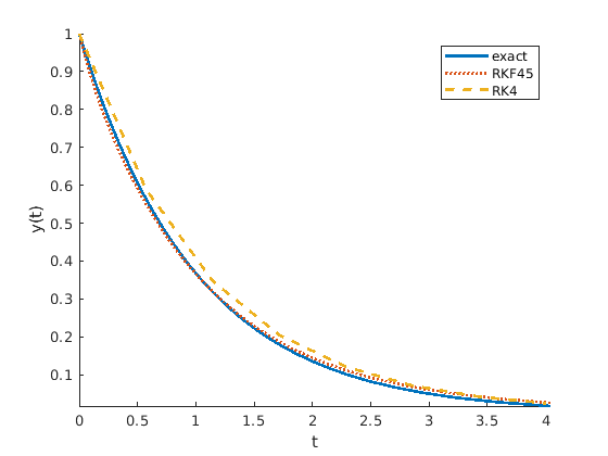
Fig. 11.19 The adjustable step size of the RKF45 algorithm gives accurate results with good performance.

11.5.7.2. MATLAB’s ode45

Although the adaptive rkf45ODE function has good results, it is not as accurate as MATLAB’s ode45 function. Using the same comparison test shown in figure Fig. 11.19, the ode45 function had a maximum error of \(6{\times}10^{-6}\), and a plot of its solution appears to be directly on top of the exact solution plot. MATLAB’s ode45 is the ODE solver that should be tried first for most problems. It has good accuracy and performance for ODEs that are not stiff. [5] Like the RKF45 method, it uses an adaptive step size algorithm based on the fourth and fifth order Runge-Kutta formula.

The ode45 function is called with the same arguments as the ODE solvers previously described, except neither the initial step size nor the number of evaluation points is given. The MATLAB ODE solvers also offer additional flexibility regarding the evaluation points. If the tspan argument contains more than two values, then tspan is taken to be a vector listing the evaluation points to use.

As before, we often save two return values from ode45, [t, y]= ode45(f, tspan, y0). The return values are stored in column vectors rather than row vectors, as with the previously used simple functions. If no return values are specified, ode45 will make a plot of the \(y\) values against the \(t\) axis.

The MATLAB ODE solvers have several additional options and tunable parameters. Rather than passing those individually to the solver, a data structure holding the options is passed as an optional argument. The data structure is created and modified using the odeset command with name–value pairs. Refer to the MATLAB documentation for odeset for a full list of the options and their descriptions.

>> options = odeset('RelTol', 1e-5);          % create
>> options = odeset(options, 'AbsTol',1e-7);  % modify
>> [t, y] = ode45(f, tspan, y0, options);     % use

11.5.8. The Logistic Equation

Let’s look at an example problem that models population growth slowed by competition, which occurs when the population has limited resources. The growth is proportional to the population size, \(y\). The competition (\(y\) against \(y\)) adds a \(-y^2\) term.

\[\frac{dy}{dt} = a\,y - b\,y^2.\]

The solution is modeled with positive and negative values for \(t\). Strang’s text on differential equations ([STRANG14], p. 55) gives the analytic solution as:

\[y(t) = \frac{a}{d\,e^{-a\,t} + b}.\]

where, \(d = \frac{a}{y(0)} - b\).

The population size is modeled as zero in the distant past (\(t = -\infty\)). The steady state (\(t = \infty\)) population size is \(K = \frac{a}{b}\), which is the sustainable population size.

The halfway point can be modeled as \(y(0) = a/2b\).

The logistic_diffEq script computes the positive half of the solution and then reflects the values to get the negative time values. The solution plot is shown in figure Fig. 11.20.

% File: logistic_diffEq.m
% Logistic Equation: a = 1, b = 1
f = @(t, y) y - y.^2;
tspan = [0 5]; y0 = 1/2;
[t, y] = ode45(f, tspan, y0);
figure, plot(t,y)
t1 = flip(-t); y1 = flip(1-y); t2 = [t1;t];
y2 = [y1;y]; analytic = 1./(1 + exp(-t2));
figure, hold on
plot(t2, y2, 'o'), plot(t2, analytic)
hold off, title('Logistic Equation')
xlabel('t'), ylabel('y')
legend('ode45 Numeric Solution', 'Analytic Solution', ...
    'Location', 'northwest');

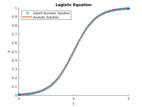
Fig. 11.20 Numerical and analytical solution to the logistic ODE

11.5.9. Stiff ODEs

A problem is stiff if the solution contains multiple terms with different step size requirements. A slower-moving component may dominate the solution; however, a less significant component may change much faster. Adaptive step size algorithms must take small steps to maintain accurate results. Because stiff ODEs have solutions with multiple terms, they come from either second-order or higher-order ODEs or systems of ODEs.

We will now look at an example of a moderately stiff system of ODE equations. Then we will see how implicit solvers solve stiff systems of ODEs and are unconditionally stable. Then we will look at MATLAB’s stiff ODE solver, ode15s.

11.5.9.1. Stiff ODE Systems

Here we show a system of ODEs that has a moderately stiff solution. See Systems of Linear ODEs for a review of systems of first-order, linear ODEs.

\[\begin{split}\left\{\begin{aligned} x' &= -25\, x + 24\, y{,}\\ y'&= 24\, x - 25\, y{,} \end{aligned}\right. \qquad \begin{aligned} x(0) &= 2 \\ y(0) &= 1 \end{aligned}\end{split}\]

It is more convenient to express systems of ODEs using vectors and matrices.

\[\begin{split}\bm{u}(t) = \begin{bmatrix} x(t) \\ y(t) \end{bmatrix} \qquad \mathbf{A} = \begin{bmatrix} -25 & 24 \\ 24 & -25 \end{bmatrix} \qquad \bm{u'} = \mathbf{A}\,\bm{u} \qquad \bm{u}_0 = \begin{bmatrix} 1 \\ 2 \end{bmatrix}\end{split}\]

The eigenvectors, eigenvalues, and \(c\) coefficients are found with some help from MATLAB.

\[\begin{split}\bm{x}_1 = \frac{1}{\sqrt{2}}\begin{bmatrix} 1 \\ -1 \end{bmatrix} \quad \bm{x}_2 = \frac{1}{\sqrt{2}}\begin{bmatrix} 1 \\ 1 \end{bmatrix} \quad \begin{array}{clcl} {\;} & {\lambda_1 = -49} & {\;} & {c_1 = -\sqrt{2}\cdot 0.5} \\ {\;} & {\lambda_2 = -1} & {\;} & {c_2 = \sqrt{2}\cdot 1.5} \end{array}\end{split}\]

The solution to the system of ODEs then comes from the general solution for systems of first order, linear ODEs as given by equation (8.10) in Systems of Linear ODEs.

(11.9)\[\bm{u}(t) = c_1 e^{\lambda_1\,t}\bm{x}_1 + c_2 e^{\lambda_2\,t}\bm{x}_2\]

(11.10)\[\begin{split}\bm{u}(t) = \left\{\begin{aligned} x(t) &= -0.5\, e^{-49\,t} + 1.5\, e^{-t} \\ y(t) &= 0.5\, e^{-49\,t} + 1.5\, e^{-t} \end{aligned}\right.\end{split}\]

The system given by equation (11.10) is stiff because the exact solution has terms with significantly different exponent values coming from the eigenvalues of \(\bf{A}\). The stability constraints on the \(e^{-49\,t}\) terms require \(h < 2/49 \approx 0.0408\). From the beginning of the evaluation, those terms will move toward zero much faster than the \(e^{-t}\) terms. We can see from figure Fig. 11.21 and figure Fig. 11.22 that an adaptive algorithm such as RKF45 or MATLAB’s ode45 will significantly reduce the step size from the beginning of the evaluations until the \(e^{-49\,t}\) term has sufficiently gone to zero. The errors between the adaptive solution and the exact solution eventually go to near zero, and the step sizes get larger.

>> % Code for figures 11.21 and 11.22
>> A = [-25 24; 24 -25]; u0 = [1;2];
>> fA = @(t, u) A*u;
>> [t, u] = rkf45ODE(fA, [0 1], u0, 0.04);
>> x = @(t) -0.5*exp(-49*t) + 1.5*exp(-t);
>> y = @(t) 0.5*exp(-49*t) + 1.5*exp(-t);

>> figure, hold on
>> plot(t, u(1,:), 'o'), plot(t, u(2,:), '+')
>> plot(t, x(t), ':'), plot(t, y(t), '--')
>> hold off

>> U = [x(t); y(t)];
>> figure, hold on
>> plot(t, vecnorm(U - u))
>> plot(t(1:end-1), diff(t), 'o:')
>> hold off

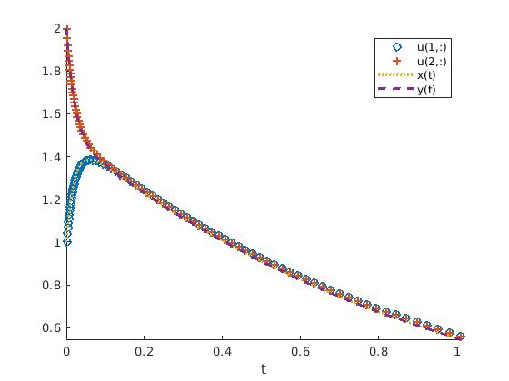
Fig. 11.21 Stiff ODE system—the \(\pm 0.5\,e^{-49\,t}\) terms quickly go to zero and the \(x(t)\) and \(y(t)\) solutions approximately merge to \(1.5\,e^{-t}\).

Fig. 11.22 Error and step size for stiff ODE system. First curve—the norm of the error vector between the exact solution and that found from the RKF45 solver. Second curve—the step size, \(h\), for the stiff ODE system.

11.5.9.2. Implicit Solvers for Systems of ODEs

The implicit backward Euler (IBE) method is used here to solve stiff systems of ODEs. The initial discussion parallels that of Implicit Backward Euler Method, but the equations are extended to systems of ODEs. As with the implicit solver for a single ODE equation, the IBE method for systems of ODEs is also unconditionally stable.

We will again use the decaying exponential ODE from the previous section. The \(\bf{A}\) matrix is required to have real, negative eigenvalues.

\[\bm{u'}(t) = \mathbf{A}\,\bm{u}(t) \qquad \bm{u}(0) = \bm{u}_0\]

The solution is \(\bm{u}(t) = \bm{u}_0 e^{\mathbf{A}\,t}\). Refer to Systems of Linear ODEs and A Matrix Exponent and Systems of ODEs for more information about how we get from a solution with a matrix in the exponent to equation (11.9).

Notice that we do not have a negative sign in front of the \(\bf{A}\) matrix as we previously saw with \(a\) in the scalar ODE from Stability Constraints. But a decaying exponential goes to zero when \(t\) goes to infinity because the eigenvalues of \(\bf{A}\) are negative.

We get the starting equation for the numerical solution by applying equation (11.7).

\[\bm{u}_k = \bm{u}_{k+1} - h\,\mathbf{A}\,\bm{u}_{k+1} = (\mathbf{I} - h\,\mathbf{A})\,\bm{u}_{k+1}\]

(11.11)\[\bm{u}_{k+1} = (\mathbf{I} - h\,\mathbf{A})^{-1}\,\bm{u}_k\]

Equation (11.11) is an implicit equation for solving systems of ODEs numerically, and is implemented in the IBEsysODE function. Notice that the implicit approach requires solving an equation at every step. In this case, the equation is a linear system of equations with a fixed matrix. Hence, the IBEsysODE function uses LU decomposition once and calls on MATLAB’s triangular solver via the left-divide operator to quickly find a solution in each loop iteration. If this were a nonlinear problem, then numerical methods such as Newton’s method or the secant method described in Numerical Roots of a Function would be needed, which could add significant computation. For this reason, implicit methods are not recommended for problems that are either not stiff or nonlinear [SHEN15].

function [t, u] = IBEsysODE(A, tspan, u0, n)
% IBESYSODE - ODE solver using the Implicit Euler Backward
%             method for systems of ODEs.
%
%   A - matrix defining the system coefficients
%   tspan - row vector [t0 tf] for initial and final time
%   y0 - initial value of y
%   n - number of y values to find
    h = (tspan(2) - tspan(1))/n;
    t = linspace(tspan(1), tspan(2), n);
    m = size(A, 1); u = zeros(m, n); u(:,1) = u0;
    [L, U, P] = lu(eye(m) - h*A);
    for k = 1:n-1
        u(:,k+1) = U\(L\(P*u(:,k)));
    end

Figure Fig. 11.23 shows the numerical solution that the IBEsysODE function found for our stiff system of ODEs. Since this is a fixed step size solution, the step size was decreased to 0.02 to track the quickly changing \(e^{-49\,t}\) terms in the solution. Of course, the small step size is not needed once the \(e^{-49\,t}\) term is sufficiently close to zero. Remember that there is a difference between accuracy and stability. A lack of stability causes the solution to be wrong as \(k \to \infty\). A lack of accuracy means that the exact solution is not well modeled by the numerical solution, which is often solved by reducing the step size.

>> A = [-25 24; 24 -25];
>> u0 = [1;2];
>> [t, u] = IBEsysODE(A, [0, 1], u0, 50);
>> x=@(t)-0.5*exp(-49*t) + 1.5*exp(-t);
>> y=@(t)0.5*exp(-49*t) + 1.5*exp(-t);
>> figure, hold on
>> plot(t, u(1,:), 'o')
>> plot(t, u(2,:), '+')
>> plot(t, x(t), ':')
>> plot(t, y(t), '--')
>> hold off

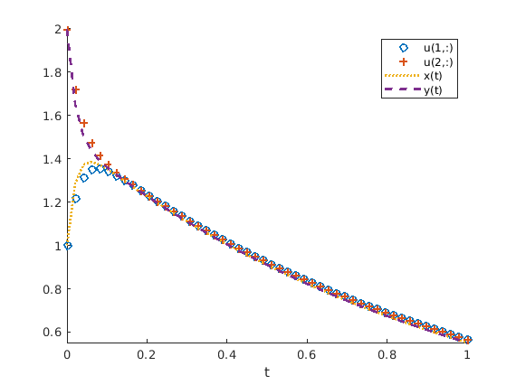
Fig. 11.23 With enough data points, the IBEsysODE function is able to to reasonably well track the rapidly changing solution of the \(e^{-49\,t}\) terms.

To evaluate the stability of the IBE method, we start by using induction to express the steady state solution in terms of the initial value.

\[\bm{u}_k = \left[(\mathbf{I} - h\,\mathbf{A})^{-1}\right]^k\,u_0\]

The stability constraint is that \(\bm{u}_k \to 0\) as \(k \to \infty\). So we need that

\[\norm{(\mathbf{I} - h\,\mathbf{A})^{-1}}_2 < 1, \; \text{ for all }h.\]

Since our \(\bf{A}\) matrix is symmetric, we can use the property of \(\norm{\cdot}_2\) matrix norms that \(\norm{\mathbf{A}}_2 = \max_i \abs{\lambda_i(\mathbf{A})}\), where \(\lambda_i(\mathbf{A})\) means the \(i\)th eigenvalue of \(\bf{A}\) (Matrix Norms).

\[\max_i \abs{\lambda_i\left((\mathbf{I}-h\,\mathbf{A})^{-1}\right)} < 1\]

Now we can make use of the eigenvalue property for symmetric matrices that \(\lambda_i(\mathbf{A}^{-1}) = \frac{1}{\lambda_i(\mathbf{A})}\) (equation (8.4) in Properties of Eigenvalues and Eigenvectors).

\[\max_i\, \abs{\frac{1}{\lambda_i(I - h\,\mathbf{A})}} < 1\]

(11.12)\[\min_i\, \abs{\lambda_i(I - h\,\mathbf{A})} = \min_i\, \abs{1 - h\,\lambda_i(\mathbf{A})} > 1\]

Equation (11.12) holds for any symmetric \(\bf{A}\) matrix with negative eigenvalues. So the implicit backward Euler method is unconditionally stable for systems of ODEs.

Unconditionally stable ODE solving algorithms remove the concern about having an unstable numerical solution because the step size is too large, but as we saw in figure Fig. 11.23, accuracy requirements may still require a reduced step size. The more complex and robust algorithms of MATLAB’s ODE solvers for stiff systems can adjust the step size enough to find accurate solutions without being excessively slowed by a stiff system.

11.5.9.3. MATLAB’s ode15s

MATLAB has several stiff ODE solvers. The ode15s function should be tried first for stiff ODEs. The primary authors of MATLAB’s suite of ODE solvers, Shampine and Reichelt, describe ode15s as an implicit quasi-constant step size algorithm. They further give the following suggestion regarding picking which ODE solver to use [SHAMPINE97].

\(\ldots\) Except in special circumstances, ode45 should be the code tried first. If there is reason to believe the problem to be stiff, or if the problem is unexpectedly difficult for ode45, the ode15s code should be tried.

Figure Fig. 11.24 shows how ode15s handles the stiff system of ODEs used in the previous examples.

>> % Code for figure 11.24
>> A = [-25 24; 24 -25]; u0 = [1;2];
>> fA = @(t, u) A*u;
>> [t, y_ode15s] = ode15s(fA, [0 1], u0);
>> t = t'; u = y_ode15s';
>> x = @(t) -0.5*exp(-49*t) + 1.5*exp(-t);
>> y = @(t) 0.5*exp(-49*t) + 1.5*exp(-t);
>> figure, hold on
>> plot(t, u(1,:)', 'o'), plot(t, u(2,:)', '+')
>> plot(t, x(t), ':'), plot(t, y(t), '--')
>> hold off

Fig. 11.24 The ode15s ODE solver is designed for stiff systems, so the less significant, but rapidly changing terms do not significantly reduce the step size.

11.5.10. MATLAB’s Suite of ODE Solvers

MATLAB’s ode45 and ode15s are the recommended nonstiff and stiff ODE solvers for most problems. If those do not give satisfactory results, then ode23 and ode113 might be tried for nonstiff problems. For stiff problems, ode23s should be the next function tried after ode15s. Additional documentation and research may be needed to select the best solver for some problems. The MathWorks’ web pages have quite a bit of documentation on the suite of ODE solvers. The MATLAB Guide by Higham and Higham [HIGHAM17] have extended coverage of MATLAB’s ODE solvers. The MATLAB ODE solvers lists MATLAB’s suite of ODE solvers.

Table 11.1 The MATLAB ODE solvers

Solver	Problem type	Description
ode45	Nonstiff	Explicit Runge-Kutta, orders 4 and 5
ode23	Nonstiff	Explicit Runge-Kutta, orders 2 and 3
ode113	Nonstiff	Explicit linear multistep, orders 1–13
ode15s	Stiff	Implicit linear multistep, orders 1–5
ode15i	Fully implicit	Implicit linear multistep, orders 1–5
ode23s	Stiff	Modified Rosenbrock pair, orders 2 and 3
ode23t	Mildly stiff	Implicit trapezoid rule, orders 2 and 3
ode23tb	Stiff	Implicit Runge-Kutta, orders 2 and 3

Online Resources

• This MathWorks web page has some good tutorial videos about numerical solutions to differential equations. Although the ODE solvers in MATLAB are more complex than the algorithms demonstrated in the first three videos, they explain the basic concepts.

• MATLAB’s ODE solvers are reviewed on this MathWorks website.

function [t, y] = rkf45ODE(f, tspan, y0, h0)
% rk5ODE - Adaptive interval ODE solver using the
%          Runge-Kutta-Fehlberg method.
%
%   f - vectorized derivative function, y' = f(t, y)
%   tspan - row vector [t0 tf] for initial and final time
%   y0 - initial value of y, scalar or column vector
%   h0 - initial step size
    tol = 2e-5;
    h = h0;
    nEst = ceil((tspan(2) - tspan(1))/h);
    m = size(y0, 1);
    t = zeros(1, 2*nEst);  % estimated preallocation
    y = zeros(m, 2*nEst);
    z = zeros(m, 2*nEst);
    t(1) = tspan(1);
    y(:,1) = y0;      % RKF45 results
    z(:,1) = y0;      % RK4 results
    k = 1;
    while t(k) < tspan(2)
        s1 = h*f(t(k), y(:,k));
        s2 = h*f(t(k) + h/4, y(:,k) + s1/4);
        s3 = h*f(t(k) + h*3/8, y(:,k) + s1*3/32 + s2*9/32);
        s4 = h*f(t(k) + h*12/13, y(:,k) + s1*1932/2197 ...
            - s2*7200/2197 + s3*7296/2197);
        s5 = h*f(t(k) + h, y(:,k) + s1*439/216 - s2*8 ...
            + s3*3680/513 - s4*845/4104);
        s6 = h*f(t(k) + h/2, y(:,k) - s1*8/27 + s2*2 ...
            - s3*3544/2565 + s4*1859/4104 - s5*11/40);
        z(:,k+1) = y(:,k) + s1*25/216 + s3*1408/2565 ...
            + s4*2197/4101 - s5/5;  % RK4
        y(:,k+1) = y(:,k) + s1*16/135 + s3*6656/12825 ...
            + s4*28561/56430 - s5*9/50 + s6*2/55; % RKF5
        % no divide by 0, h at most doubles
        algDiff = max(tol/32, norm(z(:,k+1) - y(:,k+1)));
        s = (tol/(2*algDiff))^0.25;
        h = h*s;
        if s > 0.84
            t(k+1) = t(k) + h;
            k = k + 1;
        end
    end
    % delete unused preallocated memory
    t(k+1:end) = []; y(:,k+1:end) = [];

Footnotes:

[1]

This is the forward Euler method. A variant of this algorithm is the implicit backward Euler method, which we will use in Implicit Backward Euler Method.

[2]

We use \(t\) for time as a variable of the ODE function, but a spatial variable, such as \(x\), could also be used.

[3]

Stiff ODEs are addressed in Stiff ODEs.

[4]

\(h = \frac{(20 - 0)}{(n - 1)}\), \(h = 5\), so \(n = 5\).

[5]

Stiff ODEs are addressed in Stiff ODEs.