11.4. Numerical Integration¶

Numerical integration is an important numerical method because analytic solutions are often not available. Surprisingly, the seemingly simple equation $y = e^{-x^2}$ can not be integrated analytically.

Fig. 11.12 shows that the value of a definite integral is the area bounded by the function, the $x$ –axis, and the lower and upper bounds of the integral.

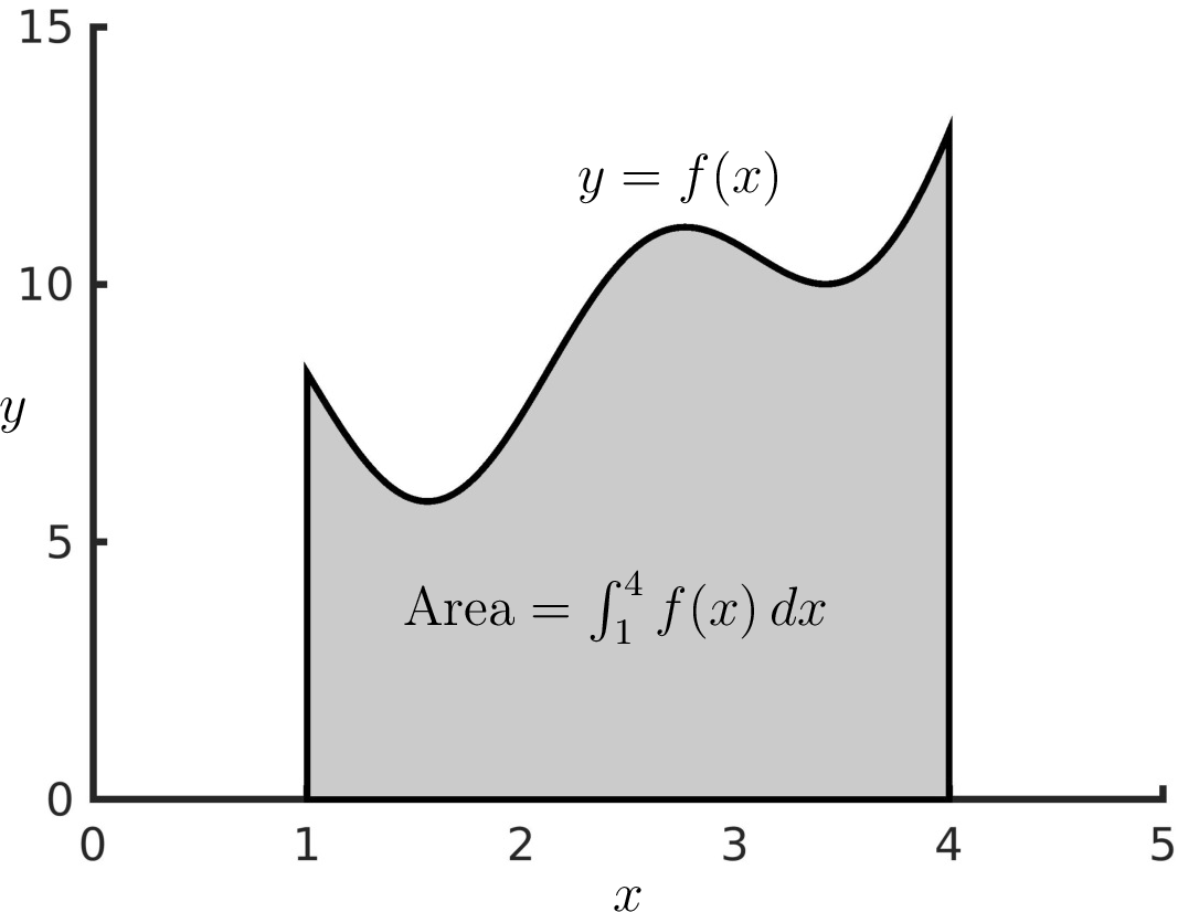
Fig. 11.12 A definite integral is an area calculation.

Numerical techniques estimate the area by summing the areas of a sequence of thin slices (subintervals). You may remember three such techniques from calculus class. The Reimann Integral uses rectangular regions to estimate the area of each small subinterval. The Trapezoid Rule improves the results by modeling the area of each subinterval as a trapezoid. Simpson’s Rule provides a more accurate estimate by modeling the curve over a pair of subintervals as a quadratic polynomial.

11.4.1. MATLAB’s Integral Function¶

MATLAB has a function for computing definite integrals called integral, which is a replacement for an older function called quad. The integral function uses a global adaptive quadrature algorithm where the integration region is divided into piecewise smooth regions before integrating each subinterval. The widths of the subintervals are adapted so that each subinterval is accurately modeled by an equation.

The integral function is called with arguments of a function handle and the interval of the integral (I = integral(f, a, b)). Be sure to use element-wise arithmetic operators when defining the function so that it can accept and return vectors. The integration interval is normally specified with a pair of real scalars, but negative and positive infinity (-Inf and Inf) may be used. See MATLAB’s documentation for information about complex functions, and the use of tolerances and waypoints.

Here are a few usage examples.

>> integral(@(x) sin(x), 0, pi)
ans =
    2.0000
>> integral(@(x) exp(-2*x), 0, Inf)
ans =
    0.5000
>> f = @(x) x.^2 - 5.*x + 8;
>> integral(f, 1, 4)
ans =
    7.5000

11.4.2. Fixed Width Subinterval Algorithms¶

Although, one only needs MATLAB’s integral function to compute integrals numerically, it is desirable to learn the basics of the numeric integration algorithms. Knowledge of the algorithms not only helps one to better understand and appreciate MATLAB’s functions, but may be needed to write an integration function in a programming language, such as C, where MATLAB’s functions are not available. We will consider how to implement numeric integration algorithms using the trapezoid rule and Simpson’s rule. We do not discuss results from Reimann integrals because integrals from trapezoids are only slightly more complex than Reimann integrals, but are more accurate.

11.4.2.1. Trapezoid Rule Integrals¶

The geometry of a trapezoid is illustrated in Fig. 11.13. When an integration region is divided into equal width trapezoids separated by grid points $\{x_1, x_2, \ldots, x_n \}$ , then the width of each trapezoid is $h = x_{i+1} - x_i$ . The area the trapezoid is the product of the width with the average height of the two sides.

$\text{Area} = h\,\frac{f(x_i) + f(x_{i+1})}{2}$

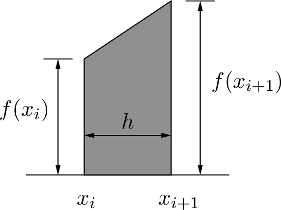
Fig. 11.13 The shape of a trapezoid and its size measurements.

The definite integral of a function over a region from $a$ to $b$ is approximated by the sum of trapezoids found by splitting the region into $n - 1$ equal width subintervals, where $n$ is the number of grid points that divide the interval into subintervals.

$h = \frac{b - a}{n - 1}$

$\int_{a}^{b} f(x)\,dx \approx \sum_{i=1}^{n - 1} h\,\frac{f(x_i) + f(x_{i+1})}{2}$

In the summation, each term except the first and last appear twice because they are part of the calculation of two trapezoids.

$\int_{a}^{b} f(x)\,dx \approx \frac{h}{2} \left(f(x_1) + 2\sum_{i=2}^{n - 1} f(x_i) + f(x_n) \right)$

As shown in Fig. 11.14, the area of each trapezoid is sometimes more, less, or nearly the same as the true area of each subinterval. Using more subintervals, which reduces the size of $h$ , will improve the accuracy. With narrower subintervals, the spanned region of $f(x)$ from $x_i$ to $x_{i+1}$ will more closely resemble a straight line. Of course, we need to be sensitive to the size of $h$ to avoid excessive round-off errors that can occur when $h$ is very small.

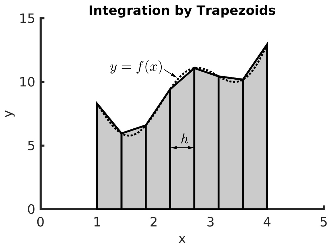
Fig. 11.14 The trapezoid rule models each subinterval as a trapezoid. The definite integral is the sum of the trapezoid areas.

The following function implements the trapezoid rule to calculate an estimate of a definite integral.

function I = trapIntegral(f, a, b, n)
% TRAPINTEGRAL - Definite integral by trapezoid area summation.
%
% f - vector aware function
% a - lower integration boundary
% b - upper integration boundary, a < b
% n - number of subinterval trapezoids

    if a >= b
        error('Variable b should be greater than a.')
    end
    h = (b - a)/n;
    x = linspace(a, b, n+1);
    y = f(x);
    I = (h/2)*(y(1) + 2*sum(y(2:end-1)) + y(end));

Testing of the trapezoid rule integration function shows that it finds an answer that is somewhat close with a modest number of grid points, but struggles to find the true definite integral value even as the number of grid points is increased.

>> fun = @(x) x.^2;
>> trapIntegral(fun, 0, 4, 10)  % correct = 21.3333
ans =
   21.4650
>> trapIntegral(fun, 0, 4, 50)
ans =
   21.3378
>> trapIntegral(fun, 0, 4, 100)
ans =
   21.3344

>> f = @(x) x.^2 - 3.*x + 2*sin(3*x).*exp(-0.01*x) + 10;
>> trapIntegral(f, 1, 4, 10)    % correct = 27.30753
ans =
   27.4644
>> trapIntegral(f, 1, 4, 100)
ans =
   27.3088
>> trapIntegral(f, 1, 4, 500)
ans =
   27.3076

11.4.2.2. Simpson’s Rule Integrals¶

Rather than using a straight line to approximate the function over an integration subinterval, Simpson’s rule estimates the function as a parabola represented with a quadratic equation. Each integration region consists of two adjacent subintervals and three grid point. The three grid points are used to find the quadratic equation from which the area is computed. The development of the quadratic equation is covered in Calculus textbooks and can also be found on several web pages. It is typically found from a Taylor series expansion of a quadratic equation or using Lagrange polynomial interpolation [SIAUW15].

Lagrange polynomial interpolation finds a polynomial that goes through a set of data points. The Lagrange polynomial, $P(x)$ , has the property that $P(x_i) = y_i$ for all given $(x_i, y_i)$ data points. We first find a Lagrange basis polynomial, $P_i(x)$ , for each of given $x_i$ value. The basis polynomials are products of factors such that $P_i(x_i) = 1$ and $P_i(x_j) = 0$ when $i \neq j$ . Then the Lagrange polynomial is a sum of products between the basis polynomials and the given $y_i$ values. The properties of the basis polynomials ensure that the Lagrange polynomial passes through each point.

$P_i(x) = \prod_{j=1, j\neq i}^n \frac{x - x_j}{x_i - x_j}$

$P(x) = \sum_{i=1}^n y_i\,P_i(x)$

Lagrange Polynomial Example

Let us use Lagrange polynomial interpolation to find the quadratic equation that passes through the points $\{(0, 2), (1, 5), \text{and} (2, 6)\}$ .

$\begin{array}{rl} P_1(x) &= \frac{(x - x_2)(x - x_3)}{(x_1 - x_2)(x_1 - x_3)} = \frac{(x - 1)(x - 2)}{(0 - 1)(0 - 2)} = \frac{1}{2}(x^2 - 3\,x + 2) \\ \hfill \\ P_2(x) &= \frac{(x - x_1)(x - x_3)}{(x_2 - x_1)(x_2 - x_3)} = \frac{(x - 0)(x - 2)}{(1 - 0)(1 - 2)} = -x^2 + 2\,x \\ \hfill \\ P_3(x) &= \frac{(x - x_1)(x - x_2)}{(x_3 - x_1)(x_3 - x_2)} = \frac{(x - 0)(x - 1)}{(2 - 0)(2 - 1)} = \frac{1}{2}(x^2 - x) \end{array}$

$\begin{array}{rl} P(x) &= 2\,P_1(x) + 5\,P_2(x) + 6\,P_3(x) \\ &= (1 - 5 + 3)\,x^2 + (- 3 + 10 - 3)\,x + 2 \\ &= -x^2 + 4\,x + 2 \end{array}$

>> P = @(x) -x.^2 + 4*x + 2;
>> x = linspace(-1, 3);
>> y = P(x);
>> plot(x,y)
>> hold on
>> plot([0 1 2], [2 5 6], 'd', 'MarkerSize', 10)
>> hold off

Fig. 11.15 The Lagrange polynomial goes through the data points $\{(0, 2), (1, 5), \text{and} (2, 6)\}$ .

Fig. 11.16 illustrates one region of integration. The quadratic equation $P(x)$ passes through the three points $\{(x_{i-1}, f(x_{i-1})), (x_{i}, f(x_{i})), \text{and} (x_{i+1}, f(x_{i+1}))\}$ , which are the intersections between the three grid points and $f(x)$ . Using integration by substitution and some algebra, the definite integral of each integration region is given by

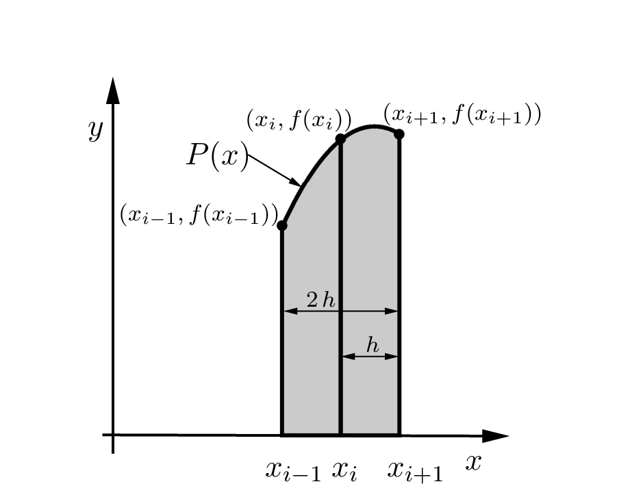
$I_i = \int_{x_{i-1}}^{x_{i+1}} P(x)\,dx = \frac{h}{3}\left(f(x_{i-1}) + 4\,f(x_i) + f(x_{i+1})\right).$

Fig. 11.16 Simpson’s Rule subinterval region of integration.

Then the definite integral from $a$ to $b$ is approximated by the sum of the subinterval integrals. Since each subinterval integral spans two subintervals, the count of function values at even and odd grid points are not the same.

$\int_a^b f(x)\,dx \approx \frac{h}{3}\left(f(x_1) + 4\left(\sum_{i = 2,\, i\, \text{even}}^{n - 1} f(x_i)\right) + 2\left(\sum_{i = 3,\, i\, \text{odd}}^{n - 2} f(x_i)\right) + f(x_n)\right).$

Fig. 11.17 shows that Simpson’s rule can find accurate definite integral results if the subintervals are small enough to accurately model the function with quadratic equations.

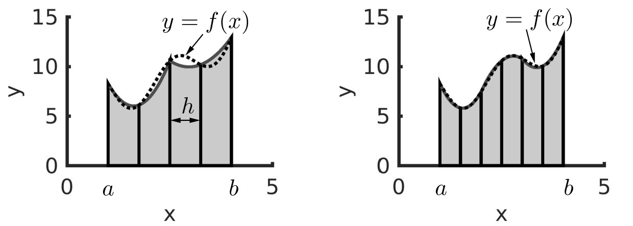
Fig. 11.17 Left: Simpson rule integration with 5 grid points, 4 subintervals, and 2 integration regions. Right: Simpson rule integration with 7 grid points, 6 subintervals, and 3 integration regions.

Note

Because Simpson’s rule computes integrals over two subintervals, the number of subintervals must be an even number. So the number of grid points must be an odd number. To satisfy the indexing requirements of the sum functions, the minimum number of grid points is 5.

The simpsonIntegration function implements Simpson’s rule integration.

function I = simpsonIntegral(f, a, b, n)
% SIMPSONINTEGRAL - Definite integral by Simpson's rule.
%
% f - vector aware function
% a - lower integration boundary
% b - upper integration boundary, a < b
% n - number of subintervals, must be an even number and >= 4

    if a >= b
        error('Variable b should be greater than a.')
    end
    if mod(n, 2) ~= 0 || n < 4
        error('Variable n, should be an even number, n >= 4.')
    end
    h = (b - a)/n;
    x = linspace(a, b, n+1);
    y = f(x);
    I = (h/3)*(y(1) + 4*sum(y(2:2:end-1)) + 2*sum(y(3:2:end-2)) + y(end));
    % MATLAB indexing starts at 1, so even and odd are reversed.

Testing results show that Simpson’s rule integration is more accurate than trapezoid integration even with fewer grid points.

>> fun = @(x) x.^2
>> simpsonIntegral(fun, 0, 4, 8)
ans =           % correct = 21.3333
   21.3333

>> f = @(x) x.^2-3.*x+2*sin(3*x).*exp(-0.01*x)+10
>> simpsonIntegral(f, 1, 4, 8)
ans =           % correct = 27.30753
   27.2950
>> simpsonIntegral(f, 1, 4, 18)
ans =
   27.3071
>> I = simpsonIntegral(f, 1, 4, 28)
I =
   27.3075
>> error = abs(I - integral(f, 1, 4))
error =           % compare to MATLAB's integral
    7.1945e-05

11.4.3. Recursive Adaptive Integral¶

The following recursive function investigates the concept of an adaptive algorithm, like MATLAB’s integral function, that adjusts the width of each subinterval based the accuracy of intermediate results. The basic concept of how the algorithm works is simple. If the function to be integrated fits the integration model (trapezoid or quadratic equation) over the integral region, then we have an accurate definite integral. However, if the integration model is a poor data fit, then the interval is divided into smaller subintervals.

For each interval, the algorithm splits the interval from $a$ to $b$ in half and calculates the area of three intervals. The interval from $a$ to $b$ is divided equally into subintervals from $a$ to $c$ and from $c$ to $b$ . If the area from $a$ to $b$ is within a small tolerance of the sum of the areas of the subintervals, then the algorithm is satisfied with the area of the interval. If not, then each subinterval is treated as its own interval and the algorithm repeats. The algorithm continues to split each subinterval until the integration model accurately fits the function over the subinterval. The returned subinterval areas are added together to find the definite integral of the function from $a$ to $b$ .

For convenience of comparisons, the adaptive function can use either the trapezoid rule or Simpson’s rule algorithms. The second argument should be either 't' or 's' to select the integration algorithm.

function I = adaptIntegral(f, intFun, a, b)
% ADAPTINTEGRAL - Adaptive interval definite integral.
%
% f - vector aware function
% intFun - 't' for trapIntegral or 's' for simpsonIntegral
% a - lower integration boundary
% b - upper integration boundary, a < b
%
% This code just demonstrates adaptive intervals.
% Use MATLAB's integral function, not this function.

    if a >= b
        error('Variable b should be greater than a.')
    end
    tol = 1e-12;
    c = (a + b)/2;

    % Three integrals
    if intFun == 't'
        Iab = trapIntegral(f, a, b, 2);
        Iac = trapIntegral(f, a, c, 2);
        Icb = trapIntegral(f, c, b, 2);
    elseif intFun == 's'
        Iab = simpsonIntegral(f, a, b, 4);
        Iac = simpsonIntegral(f, a, c, 4);
        Icb = simpsonIntegral(f, c, b, 4);
    else
        error("Specify 's' or 't' for intFun")
    end

    if abs(Iab - (Iac + Icb)) < tol
        I = Iac + Icb;
    else
        I = adaptIntegral(f, intFun, a, c) ...
            + adaptIntegral(f, intFun, c, b);
    end

Testing shows that the adaptive interval algorithm is an accurate estimator of definite integrals. Results from using Simpson’s rule are more accurate than using the trapezoid rule algorithm.

>> f = @(x) x.^2-3.*x+2*sin(3*x).*exp(-0.01*x)+10
>> I = integral(f, 1, 4);   % compare to built-in
>> I - adaptIntegral(f, 's', 1, 4)
ans =
   2.4833e-12
>> I - adaptIntegral(f, 't', 1, 4)
ans =
  -2.9574e-09

>> s = @(x) sin(x);
>> adaptIntegral(s, 's', 0, pi)
ans =
   2.0000
>> 2 - ans
ans =
  -1.2683e-12
>> 2 - adaptIntegral(s, 't', 0, pi)
ans =
   1.7330e-09

11.4. Numerical Integration¶

11.4.1. MATLAB’s Integral Function¶

11.4.2. Fixed Width Subinterval Algorithms¶

11.4.2.1. Trapezoid Rule Integrals¶

11.4.2.2. Simpson’s Rule Integrals¶

11.4.3. Recursive Adaptive Integral¶

Table of Contents

Previous topic

Next topic

This Page