11.3. Numerical Differentiation
Computing a derivative numerically is typically not difficult and can yield accurate results. To achieve the desired accuracy, we need to pay attention to the sampling rate of the data and the computer’s limits to processing very small numbers without round-off errors. Simple numerical derivative methods derive from differences of consecutive data values. We can also compute derivatives in the frequency domain for more accurate results.
11.3.1. Euler Derivative
Calculus defines the derivative of \(y(x)\) with respect to \(x\) as
For discretely sampled data, this becomes an approximation.
The variable \(h\) represents the \(x\) distance between the samples (\(\delta x\)) and is proportional to the error, which may be acceptable for some applications, but not others. The algorithm that makes use of the simple derivative definition is called the forward Euler finite-difference derivative.
For sampled data values, the MATLAB function diff returns the
difference between consecutive values, which is used to compute the
derivative dy_dx = diff(y)/h;. Note that the size of the array
returned by diff is one element smaller than the array passed to it.
To take the derivative of a function, first sample the data
(\(y\left(x_i\right)\)) at intervals of \(h\); then find the
differences of consecutive values with the diff function. The
challenge is to determine an appropriate value for \(h\). It should
be small enough to give good granularity. The evaluation of small
enough depends entirely on the evaluated data. However, it should not
be so small as to require excessive computation or to cause excessive
rounding errors from the division by \(h\). As a rule of thumb,
\(h\) should not be much smaller than
\(10^{-8}\) [SIAUW15]. Some testing with different
values of \(h\) may be required for some applications. The
deriv_cos script provides a starting point for experimentation. See
how changing the value of \(h\) affects the accuracy of the
numerical derivative. Figure Fig. 11.10 shows the plot
where \(h = \pi/40\).
% File: deriv_cos.m
% Derivative example, Compute the derivative of cos(x)

% sample step size, please experiment with h values
h = pi/40;
x = 0:h:2*pi;
y = cos(x);
dy_dx = diff(y)/h;
x1 = x(1:end-1);      % note one less to match dy_dx
actual_dy = -sin(x1);
error = abs(dy_dx - actual_dy);
me = max(error); ex = x1(error == me);

p1 = plot(x1, actual_dy, 'k', x1, dy_dx, 'r:');
title('Derivatives of cos(x)'); xticks(0:pi/2:2*pi);
xticklabels({'0','\pi/2','\pi','3\pi/2','2\pi'});
line([ex ex], [-1 1]);
text(ex+0.1, -0.4, 'Max error location');
legend(p1,{'analytic derivative','numeric derivative', },...
    'Location', 'northwest');
disp(['Max error = ',num2str(me)]);
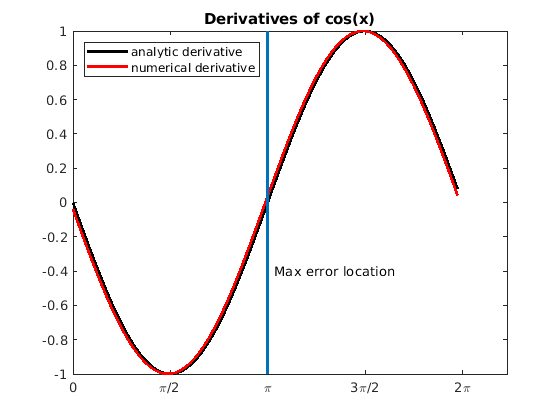
Fig. 11.10 Even though the \(h\) value is fairly large, the Euler numerical derivative of the cosine function is still close to the analytic derivative.
11.3.2. Spectral Derivative
The fast Fourier transform (FFT) provides a more accurate numerical method for estimating a derivative. The Fourier series, the Fourier transform, and the inverse Fourier transform are algorithms proposed in 1807 by the French mathematician Jean Baptiste Joseph Fourier (1768-1830) to characterize the frequencies present in continuous functions or signals. Later, the discrete Fourier transform (DFT) was used with sampled signals; however, the DFT can be rather slow for large data sets (\(\mathcal{O}(n^2)\)). Then in 1965, James W. Cooley (IBM) and John W. Tukey (Princeton) developed the fast Fourier transform (FFT) algorithm that has run-time complexity of \(\mathcal{O}(n\,\log{}n)\). The improved performance of the FFT stems from taking advantage of the symmetry found in the complex, orthogonal basis functions (\(\omega_n = e^{-2\pi i/n}\)). In our coverage, we will stick with our objective of applying the FFT for finding derivatives.
Many resources provide detailed descriptions of the Fourier transform and the FFT. The text by Brunton and Kutz provides rigorous, but still understandable, coverage [BRUNTON22], pages 53 to 70.
The FFT interests us here because of the simple relationship between the Fourier transform of a function and the Fourier transform of the function’s derivative. We can easily find the derivative in the frequency domain and then use the inverse FFT to put the derivative into its original domain.
Here, \(i\) is the imaginary constant \(\sqrt{-1}\) and \(\omega\) is the frequency in radians per second for time domain data or just radians for spatial data. We can use \(\omega = 2\pi f_s k/n\) for time domain data and \(\omega = 2\pi k/T\) for spatial domain data, where \(k\) is the sample number in the range \(\{-n/2 \text{ to } (n/2 - 1)\}\), and \(n\) is the number of data samples (usually a power of 2). The time domain data’s sampling frequency (samples/second) is \(f_s\). For spatial domain data, \(T\) is the length of the data.
The Spectral Derivative gives an example of computing the
spectral derivative using time domain data. The FFT treats frequency
data as positive and negative, so our \(\omega\) needs to do the
same. We can use our k variable to build both the time, t,
values and the frequency, w, values. The FFT and inverse FFT
algorithms reordered the data, so we must use the fftshift function
to align the frequency values with the frequency domain data.
Figure Fig. 11.11 shows a plot of the time domain spectral derivative, which aligns with the analytic derivative.
%% SpectralTimeDerivative.m
%  Numerical derivative using the spectral derivative
%  (FFT-based) algorithm --  time domain data
n = 256; fs = 8000; % samples/second
T = n/fs;           % period of samples (seconds)
k = -n/2:(n/2 - 1);
t = T*k/n;          % time values
f1 = 200; f2 = 500; % Two frequency components (Hz)

% The function and its analytic derivative
f = 2*cos(2*pi*f1*t) + cos(2*pi*f2*t);
df = -4*f1*pi*sin(2*pi*f1*t) - 2*f2*pi*sin(2*pi*f2*t);

%% Derivative using FFT (spectral derivative)
fhat = fft(f);
w = 2*pi*fs*k/n;      % radians / second
omega = fftshift(w);  % Re-order fft frequencies
i = complex(0, 1);    % Define i just to be sure it is not
                      % used for something else, or could use 1i.
dfhat = i*omega.*fhat;      % frequency domain derivative
dfFFT = real(ifft(dfhat));  % time domain derivative
%% Plotting commands
figure, plot(t, f, 'b')  % derivatives too large for same plot
title('Function'), xlabel('seconds');
figure, hold on
plot(t, df, 'k', 'LineWidth',1.5)
plot(t, dfFFT,'r--','LineWidth',1.2)
legend('True Derivative',' FFT Derivative')
title('Derivatives'), xlabel('seconds');
hold off

%% Plot the power spectrum
pwr = abs(fhat).^2/n;
figure, plot(omega/(2*pi), pwr);
xlim([-800 800])
xlabel('Frequency (Hz)'), ylabel('Power'), title('Power Spectrum')
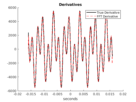
Fig. 11.11 Plot of the analytic derivative and spectral derivative of a time domain signal
