7. Least Squares Regression

See also

Here is some additional reading material on Least Squares Regression. It is one section from Gilbert Strang’s Linear Algebra textbook. ila0403.pdf

We often conduct experiments in science and engineering where we measure a system’s response as a control variable is adjusted. The measurement and control variables might be time, voltage, weight, length, volume, temperature, pressure, or any parameters relative to the system under investigation. We might expect that a polynomial equation relates the measurement and control variables, but we likely do not know the polynomial coefficients. We might not even know if the relationship between the control variable and measured data is linear, quadratic, or a higher-order polynomial. We are experimenting to learn about the system. Unfortunately, in addition to measuring the relationship between the variables, we will also measure some noise caused by the indeterminate nature of the system and measurement errors.

If the \(x\) is the control variable, the measured data can be modeled as:

\[b(x) = f(x) + n(x)\]

• \(b(x)\) is the measured data.

• \(f(x)\) is the underlying relationship we wish to find.

• \(n(x)\) is the measurement noise, which may be correlated to \(x\), or may be independent of \(x\).

The accuracy of our findings will increase with more sample points. After experimenting, we want to fit the data to a polynomial that minimizes the square of the error (\(E = \norm{\bm{e}}^2\)).

7.1. Linear Regression

In linear regression, we model the data as following a line, so we represent the relationship between the measured data points, \(\bm{b(t)}\), and the control variable, \(\bm{t}\), with line equations. The coefficients \(C\) and \(D\) are the unknowns that we need to find.

\[\begin{split}\begin{array}{c} C + D\,\bm{t} = \bm{b(t)}\\ \hfill \\ C + D\,t_1 = b(t_1) \\ C + D\,t_2 = b(t_2) \\ C + D\,t_3 = b(t_3) \\ C + D\,t_4 = b(t_4) \\ \vdots \\ C + D\,t_n = b(t_n) \end{array}\end{split}\]

Matrix \(\bf{A}\), often called the design matrix in regression terminology, defines the control variables.

\[\begin{split}\mathbf{A} = \left[ \begin{array}{ll} 1 & t_1 \\ 1 & t_2 \\ \vdots & \vdots \\ 1 & t_n \end{array} \right]\end{split}\]

Vector \(\bm{u}\) represents the unknown polynomial coefficients.

\[\begin{split}\bm{u} = \left[ \begin{array}{l} C \\ D \end{array} \right]\end{split}\]

\[\mathbf{A}\,\bm{u} = \bm{b}\]

The equations for least squares regression calculations are given in three mathematical disciplines—linear algebra, calculus, and statistics. The computations for the three are the same, but the equations look different depending on one’s vantage point.

7.1.1. Linear Algebra Based Linear Regression

Because the system of equations is over-determined, and the measured data, \(\bm{b}\), is not likely to lie in the column space of \(\bf{A}\), either the projection equations or QR decomposition may be used to approximate \(\bm{u}\) Projections Onto a Hyperplane).

\[\bm{u} = \left(\mathbf{A}^T\,\mathbf{A}\right)^{-1} \mathbf{A}^T\,\bm{b} = \mathbf{R}^{-1}\mathbf{Q}^T\bm{b}\]

The projection \(\bm{p} = \mathbf{A}\,\bm{u}\) follows directly.

7.1.2. Calculus-Based Linear Regression

The error between the projection, \(\mathbf{A}\,\bm{u}\), and the target vector, \(\bm{b}\), is \(\bm{e} = \bm{b} - \mathbf{A}\,\bm{u}\). To account for both positive and negative errors, we wish to minimize the squares of the error vector, \(E = {\norm{\bm{e}}}^{2}\).

Note that the squared length of a vector is its dot product with itself.

\[\begin{split}\begin{array}{rl} E &= \norm{\bm{b} - \mathbf{A}\,\bm{u}}^2 = (\bm{b} - \mathbf{A}\,\bm{u})^T\,(\bm{b} - \mathbf{A}\,\bm{u}) = (\bm{b}^T - \bm{u}^T\mathbf{A}^T)\,(\bm{b} - \mathbf{A}\,\bm{u}) \\ & \hfill \\ &= \bm{b}^T\bm{b} - \bm{b}^T\mathbf{A}\,\bm{u} - \bm{u}^T\mathbf{A}^T\bm{b} + \bm{u}^T\mathbf{A}^T\mathbf{A}\,\bm{u} \end{array}\end{split}\]

The minimum occurs where the derivative is zero. The derivative is with respect to the vector \(\bm{u}\), which is the gradient of \(E\). The procedure for computing the gradient is described in Appendix C of the numerical analysis text by Yang et al. [YANG05] and the vector calculus chapter of Deisenroth’s machine learning text [DEISENROTH20].

\[\nabla E = \frac{\partial E}{\partial \bm{u}} = - \mathbf{A}^T\bm{b} - \mathbf{A}^T\bm{b} + 2\mathbf{A}^T\mathbf{A}\,\bm{u} = \bm{0}\]

\[\mathbf{A}^T\mathbf{A}\,\bm{u} = \mathbf{A}^T\bm{b}\]

Calculus gives us the same equation that we get from linear algebra.

\[\bm{u} = \left(\mathbf{A}^T\mathbf{A}\right)^{-1} \mathbf{A}^T\bm{b}\]

7.1.3. Statistical Linear Regression

We start by calculating some statistical parameters from both the results, \(\bm{b}\), and the control variable, \(\bm{t}\). The equations for calculating the mean and standard deviation are found in Common Statistical Functions.

1. Mean of \(\bm{b}\) is \(\bar{\bm{b}}\).

2. Mean of \(\bm{t}\) is \(\bar{\bm{t}}\).

3. Standard deviation of \(\bm{b}\) is \(\sigma_b\).

4. Standard deviation of \(\bm{t}\) is \(\sigma_t\).

5. The correlation between \(\bm{t}\) and \(\bm{b}\) is \(r\).

   \[r = \frac{n \sum tb - \left(\sum b\right)\left(\sum t\right)} {\sigma_t\,\sigma_b}\]

We turn to statistics textbooks for the linear regression coefficients [HOGG78,MOORE18]_.

\[\begin{split}\begin{array}{l} D = \frac{r\,\sigma_b}{\sigma_t} \\ \\ C = \bar{\bm{b}} - D\,\bar{\bm{t}} \end{array}\end{split}\]

We write the matrix and vector terms as sums of the variables \(t\) and \(b\) to show that the equations for linear regression from statistics and linear algebra are the same.

\[\begin{split}\mathbf{A}^T\mathbf{A} = \begin{bmatrix} n & \sum & t \\ \sum & t & \sum & t^2 \end{bmatrix} \hspace{0.75in} \mathbf{A}^T\bm{b} = \begin{bmatrix} \sum & b \\ \sum & tb \end{bmatrix}\end{split}\]

Using elimination to solve, we get:

\[\begin{split}\left[\begin{array}{ccccc|c} n & \sum & t & \sum & b \\ \sum & t & \sum & t^2 & \sum & tb \end{array}\right]\end{split}\]

\[\begin{split}\left[\begin{array}{ccc|c} n & \sum & t & \sum & b \\ 0 & {\sum t^2 - \frac{1}{n}\left(\sum t\right)^2}{\sum tb - \frac{1}{n}\left(\sum b\right)\left(\sum t\right)} \end{array}\right]\end{split}\]

We get a match for the \(D\) coefficient by identifying statistical equations in the equation from elimination.

\[D = \frac{\sum tb - \frac{1}{n}\left(\sum b\right)\left(\sum t\right)} {\sum t^2 - \frac{1}{n}\left(\sum t\right)^2} = \frac{r\,\sigma_t\,\sigma_b}{{\sigma_t}^2} = \frac{r\,\sigma_b}{\sigma_t}\]

The \(C\) coefficient comes from back substitution of the elimination matrix.

\[C = \frac{\sum b - D\,\sum t}{n} = \bar{\bm{b}} - D\,\bar{\bm{t}}\]

7.1.4. Linear Regression Example

The linRegress script shows a simple linear regression example. The exact output differs each time the script is run because of the random noise. A plot of the output is shown in figure Fig. 7.1.

% File: linRegress.m
% Least Squares linear regression example showing the
% projection of the test data onto the design matrix A.
%
% Using control variable t, an experiment is conducted.
% Model the data as: b(t) = C + Dt.
f = @(t) 2 + 4.*t;
% A*u = b, where u = [ C D ]'
% Define the design matrix A.
m = 20; n = 2; t = linspace(-2, 3, m);
A = ones(m, n); A(:,2) = t';
b = f(t)' + 3*randn(m, 1);
u = (A'*A)\(A'*b);  % least squares line
p = A*u;            % projection vector
e = b - p;          % error vector
C = u(1); D = u(2);
fprintf('Equation estimate = %.2f + %.2f*t\n', C, D);

%% Plot the linear regression
figure, plot(t, b, 'o');
hold on, plot(t, p, 'Color', 'k');
hold off, grid on, xlabel('t'), ylabel('b')
title('Linear Regression')

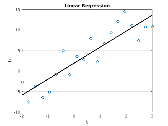
Fig. 7.1 Simple linear least squares regression. Output from the script is: Equation estimate = 1.90 + 3.89*t, which is close to the data model of \(\bm{b} = 2 + 4\,t\).

7.2. Quadratic and Higher Order Regression

Application of least squares regression to quadratic polynomials only requires adding a column to the design matrix for the square of the control variable [STRANG07].

\[\begin{split}\begin{array}{c} C + D\,t_1 + E\,t_1^2 = b(t_1) \\ C + D\,t_2 + E\,t_2^2 = b(t_2) \\ C + D\,t_3 + E\,t_3^2 = b(t_3) \\ C + D\,t_4 + E\,t_4^2 = b(t_4) \\ \vdots \\ C + D\,t_n + E\,t_n^2 = b(t_n) \end{array}\end{split}\]

\[\begin{split}\bf{A} = \left[ \begin{array}{lll} 1 & t_1 & t_{1}^{2}\\ 1 & t_2 & t_{2}^{2}\\ \vdots & \vdots & \vdots \\ 1 & t_n & t_{n}^{2} \end{array} \right]\end{split}\]

Higher-order polynomials would likewise require additional columns in the \(\bf{A}\) matrix.

The quadRegress script lists a quadratic regression example. The plot of the data is shown in figure Fig. 7.2.

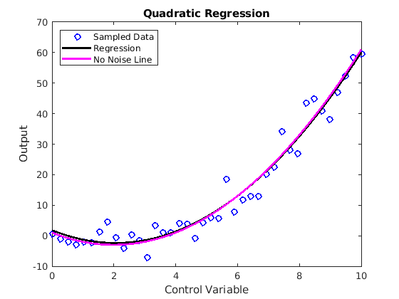
Fig. 7.2 Least squares regression fit of quadratic data. The script’s output is Equation estimate = 1.79 + -4.06*t + 0.99*t^2, which is a fairly close match to the quadratic equation without the noise.

% File: quadRegress.m
%% Quadratic Least Squares Regression Example
%
%  Generate data per a quadratic equation, add noise to it,
%  and use least squares regression to find the equation.

%% Generate data
f = @(t) 1 - 4*t + t.^2;   % Quadratic function as a handle
Max = 10; N = 40;          % number of samples
std_dev = 5;   % standard deviation of the noise
t = linspace(0, Max, N);
y = f(t) + std_dev*randn(1,N); % randn -> mean = 0, std = 1
%% Least Squares Fit to Quadratic Equation
%  model data as: b = C + Dt + Et^2
%  Projection is A*u, where u = [C D E]'
%  Determine A matrix from t.
A = ones(N,3);    % pre-allocate A - Nx3 matrix
% First column of A is already all ones.
A(:,2) = t';      % linear term, second column
A(:,3) = t'.^2;   % Quadratic term, third column

% b vector comes from sampled data
b = y';
u = (A'*A)\(A'*b);  % least squares equation
p = A*u;            % projection vector
e = B - p;          % error vector
C = u(1); D = u(2); E = u(3);
fprintf('Equation estimate = %.2f + %.2f*t + %.2f*t^2\n',C,D,E);

%% Plot the results
figure, plot(t, y, 'ob');
hold on, plot(t, p, 'k'), plot(t, f(t), 'm')
labels = {'Sampled Data', 'Regression', 'No Noise Line'};
legend(labels, 'Location', 'northwest');
hold off, title('Quadratic Regression');
xlabel('Control Variable'); ylabel('Output');

7.3. polyfit function

An erudite engineer should understand how to do least squares regression to fit a polynomial equation to a data set. However, as might be expected with MATLAB, it has a function that does the real work for us. The polyfit function does the regression calculation to find the coefficients. Then the polyval function can be used to apply the coefficients to create the \(y\) axis data points.

%% MATLAB's polyfit function
coef = polyfit(t, y, 2);
disp(['Polyfit Coefficients: ', num2str(coef)])
pvals = polyval(coef, t);

7.4. Goodness of a Fit

Statistics gives us a metric called the coefficient of determination, \(R^2\), to measure how closely a regression fit models the data. Let \(y_i\) be the data values, \(p_i\) be the regression fit values, and \(\mu\) be the mean of the data values.

\[R^2 = 1 - \frac{\sum_i (y_i - p_i)^2}{\sum_i (y_i - \mu)^2}\]

The range of \(R^2\) is from 0 to 1. If the regression fit does not align well with the data, the \(R^2\) value will be close to 0. If the model is an exact fit to the data, then \(R^2\) will be 1. In reality, it will be somewhere in between, and hopefully closer to 1 than 0.

7.5. Generalized Least Squares Regression

The key to least squares regression success is to correctly model the data with an appropriate set of basis functions. When fitting the data to a polynomial, we use progressive powers of \(t\) as the basis functions.

\[\begin{split}\begin{array}{l} f_0(t) = 1 \mbox{, a constant} \\ f_1(t) = t \\ f_2(t) = t^2 \\ \; \; \; \vdots \\ f_n(t) = t^n \end{array}\end{split}\]

The regression algorithm then uses a simple linear algebra vector projection algorithm to compute the coefficients (\(\alpha_1, \alpha_2, \ldots \alpha_n\)) to fit the data to the polynomial.

\[\begin{split}\left\{\begin{array}{rcl} \hat{y}(t_0) &=& \alpha_0\, f_0(t_0) + \alpha_1\, f_1(t_0) + \cdots + \alpha_n\, f_n(t_0) \\ \hat{y}(t_1) &=& \alpha_0\, f_0(t_1) + \alpha_1\, f_1(t_1) + \cdots + \alpha_n\, f_n(t_1) \\ &\vdots& \\ \hat{y}(t_m) &=& \alpha_0\, f_0(t_m) + \alpha_1\, f_1(t_m) + \cdots + \alpha_n\, f_n(t_m) \end{array}\right.\end{split}\]

The basis functions need not be polynomials, however. They can be any function that offers a reasonable model for the data. Consider a set of basis functions consisting of a constant offset and oscillating trigonometry functions.

\[\begin{split}\begin{array}{l} f_0(t) = 1 \mbox{, a constant} \\ f_1(t) = sin(t) \\ f_2(t) = cos(t) \end{array}\end{split}\]

The design matrix for the regression is then,

\[\begin{split}\begin{bmatrix} 1 & sin(t_0) & cos(t_0) \\ 1 & sin(t_1) & cos(t_1) \\ 1 & sin(t_2) & cos(t_2) \\ {} & \vdots & {} \\ 1 & sin(t_m) & cos(t_m) \end{bmatrix}.\end{split}\]

The genregress function implements generalized least squares regression. The basis functions are given as an input in the form of a cell array containing function handles. The trigRegress script tests the genregression function. A plot of the output is shown in figure Fig. 7.3.

% File: trigRegress.m
f = {@(x) 1, @sin, @cos};
x = linspace(-pi, pi, 1000)';
y = 0.5 + 2*sin(x) - 3*cos(x) + randn(size(x));
[alpha, curve] = genregression(f, x, y);
disp(alpha), figure, plot(x, y, 'b.')
hold on, plot(x, curve,'r', 'LineWidth', 2);
xlabel('x'), ylabel('y')
title('Regression Fit of Trig Functions')
legend('data', 'regression', 'Location', 'north')
hold off, axis tight

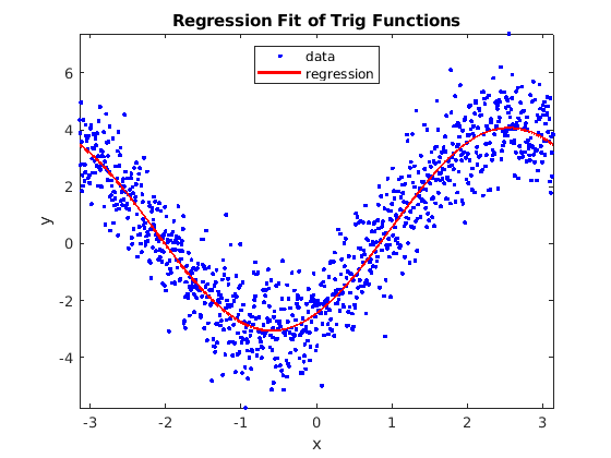
Fig. 7.3 Least squares regression of trigonometric functions

A fun application of generalized least squares is to find the Fourier series coefficients of a periodic waveform. It turns out that the regression calculation can also find Fourier series coefficients when the basis functions are sine waves of the appropriate frequency and phase. The fourierRegress script demonstrates this for a square wave. The plot of the data is shown in figure Fig. 7.4.

% File: fourierRegress.m
% Use least squares regression to find Fourier series coefficients.

f = {@(t)1,@(t) sin(t),@(t) sin(3*t),@(t) sin(5*t),@(t) sin(7*t)};
x = linspace(0, 4*pi, 1000)';
y = sign(sin(x));
% y = y + 0.1*randn(length(x),1);  % optional noise
[alpha, curve] = genregression(f, x, y);
disp(alpha), figure, plot(x, y, 'b')
hold on, plot(x, curve,'r--', 'LineWidth', 2);
xlabel('x'), ylabel('y')
title('Regression Fit of Square Wave')
legend('data', 'regression')
hold off, axis tight

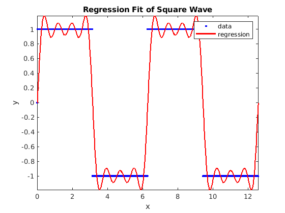
Fig. 7.4 A few terms of the Fourier series of a square wave found by least squares regression

function [ alpha, varargout ] = genregression( f, x, y )
% GENREGRESSION Regression fit of data to specified functions
%   Inputs:
%         f - cell array of basis function handles
%         x - x values of data
%         y - y values of data
%   Output:
%         alpha - Coefficients of the regression fit
%         yHat  - Curve fit data (optional)

    % A will be m-by-n, alpha and b will be n-by-1
    if length(x) ~= length(y)
        error('Input vectors not the same size');
    end
    m = length(x); n = length(f); A = ones(m,n);
    if size(y, 2) == 1 % a column vector
        b = y; cv = true;
    else
        b = y'; cv = false;
    end
    if size(x, 2) == 1 % column vector
        c = x;
    else
        c = x';
    end
    for k = 1:n
        A(:,k) = f{k}(c);
    end
    alpha = (A'*A) \ (A'*b);
    if nargout > 1
        yHat = A * alpha;
        if ~cv
            yHat = yHat';
        end
        varargout{1} = yHat;
    end
end

7.6. Fitting Exponential Data

If the data is exponential, use the logarithm function to convert the data to linear before fitting the regression data.

• The data takes the form \(y(x) = c\,e^{a\,x}\).

• Taking the logarithm of the data converts it to linear data, \(Y = log(y(x)) = log(c) + a\,x\).

• Use linear regression to find \(\hat{Y}\).

• Then \(\hat{y}(x) = e^{\hat{Y}}\).

The expRegress script shows an example of using a logarithm to facilitate least squares regression of exponential data. The plot of the output is shown in figure Fig. 7.5.

% File: expRegress.m
x = linspace(0,5); y = 25*exp(-0.5*x) + randn(1, 100);
Y = log(y); A = ones(100, 2); A(:,2) = x';
y_hat = exp(A*(A\Y'));
figure, hold on plot(x,y, 'o'), plot(x, y_hat', 'r')
hold off, legend('data', 'regression')
title('Regression Fit of Exponential Data')
xlabel('x'), ylabel('y')

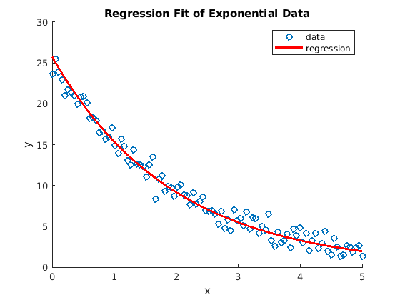
Fig. 7.5 Least squares regression of exponential data

Note

Now complete the Least Squares Regression Homework.