4.1.2. Inverse Kinematics¶

Calculating the needed joint angles that will yield a desired pose (inverse kinematics) is a more complex problem than that of forward kinematics. In some cases there may be closed form solutions, but for robots with more than a couple joints it could be very difficult, if not impossible, to derive a close form solution.

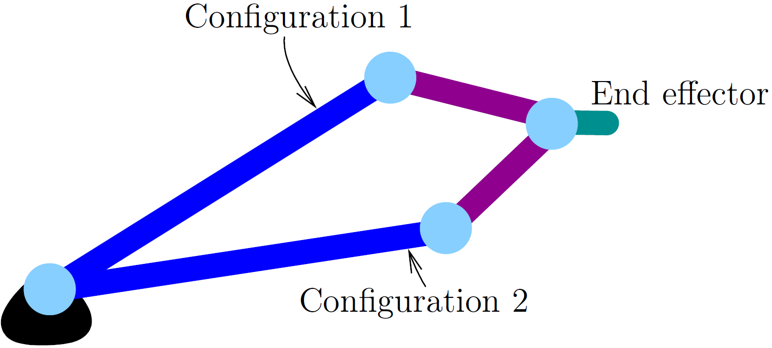
More than one set of joint angles can exist for each pose. For example, consider this simple three joint example showing two sets of joint angles with the same pose. To distinguish which pose is desired, different configurations with the same pose are often described as being either left or right handed, elbow either up or down, and wrist either flipped or not flipped.

Robot Models – Puma 560

The Robotics Toolbox by Peter Corke has models for a number of robots. Some are simple one, two, and three arm robots for the sake of learning. Others are models of real commercial robots. The Puma 560 model is used below. The Puma 560 was the first 6-axis industrial robot. It is no longer made. Because it is an old robot design, and maybe partly because it is no longer made, it is often modeled and discussed in books and classes. Some universities still have some Puma 560 robots.

>> mdl_puma560                 % create the model
% forward kinematics of a known set of joing angles
>> T = p560.fkine(qn);

% inverse kinematics - right handed, elbow up
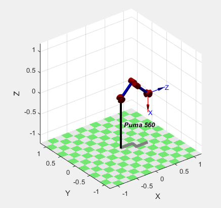
>> qn_r = p560.ikine6s(T, 'ru')
qn_r =
-0.0000    0.7854    3.1416   -0.0000    0.7854    0.0000
>> p560.plot(qn_r)

Fig. 4.4 Puma 560 robot in right handed, elbow up configuration.

% inverse kinematics - left handed, elbow up
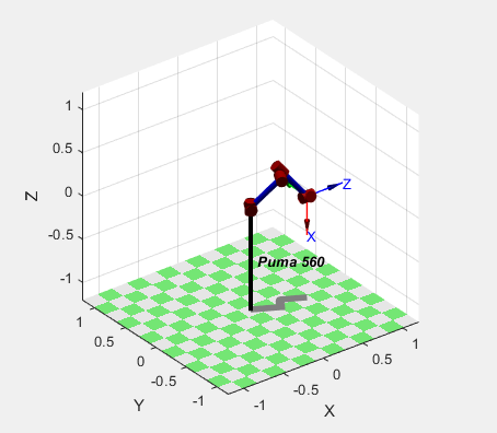
>> qn_l = p560.ikine6s(T, 'lu')
qn_l =
    2.6486   -3.9270    0.0940    2.5326    0.9743    0.3734
>> p560.plot(qn_l)

Fig. 4.5 Puma 560 robot in left handed, elbow up configuration.

4.1.2.1. Solving Inverse Kinematics Problems¶

In the example above, we used a method of the Puma 560 model to find the joint angles. There are two general approaches to solving inverse kinematic problems. In some cases, a closed form algebraic equations can be found. This is preferred because the equations can be used very quickly to find the joint angles for other poses.

This video show a trigonometry derived solution and this video shows an algebra derived solution to the inverse kinematics of a two joint robot. You can see that for even a simple robot, a closed form solution is not easy to determine.

Simplification math tricks

Use the Symbolic Math Toolbox where you can. The simplify() function is especially helpful. It knows all of the trigonometry identities.
When you see the $\sin$ and $\cos$ terms of the same angle in the equations for $x$ and $y$ , use $x^2 + y^2 = E^TE$ . There are two reasons to do this. First, some of the trigonometry functions will likely drop out because $\sin^2\theta + \cos^2\theta = 1$ . Secondly, this combines and relates the equations for $x$ and $y$ to the desired position. If $E$ is the desired position in the form of a column vector, then the dot product, $E^TE$ , is the square of the length of the vector from the origin to $E$ . The MATAB function norm returns the length of the vector ( $\sqrt{E^TE}$ ).
You may find expressions of the form $a \cos\theta + b \sin\theta = c$ . There is a known solution then for $\theta$ . Keep in mind that this returns two values for $\theta$ . The values of $\theta$ might be outside the range of $-\pi$ to $\pi$ , so use the MATLAB function wrapToPi() on the results.

$\theta = \tan^{-1}\frac{c}{\pm\sqrt{a^2 + b^2 - c^2}} - \tan^{-1}\frac{a}{b}$

When a closed form solution is not available, a numeric search algorithm can be used. MATLAB has a function called fminsearch() that uses the Nelder-Mead simplex search method. The math behind how the algorithm works is a little complicated, but you can read about it in the MATLAB documentation and articles found by searching the Internet. To use fminsearch(), one first defines a function that returns the error between the result yielded by a possible solution and the desired result. Then fminsearch() tries various possible solutions searching for a local minimum error.

A common application of fminsearch is to define a function handle that computes an error function that we wish to minimize. An example of that follows. We can use matrix multiplication to calculate the final position of a serial-link robotic arm. We can then use fminsearch to calculate the inverse kinematics of a robot, which finds the joint angles needed to position the robot end effector at a specified location. For robots with only a few joints, it may be possible to find an analytic inverse kinematic solution, but more complex robots often require numerical methods to find the desired joint angles. Multiple joint angle sets can position the robot arm at the same location. For example, we can consider either elbow-up or elbow-down configurations. Thus, the starting point value is critical for finding the desired joint angles.

Here is a simple example for a robot with two joints and two rigid arm segments (a and b). The minimized function finds the length of the error vector between forward kinematic calculation and the desired location of the end effector.

% File: fminsearch2.m
% Script using fminsearch for inverse kinematic
% calculation of a 2 joint robot arm.
E = [5.4 4.3]';
error = @(Q) norm(E - fwdKin(Q));
Qmin = fminsearch(error, [0 0]);
disp(['Q = ', num2str(Qmin)]);
disp(['Position = ', num2str(fwdKin(Qmin)')]);

function P = fwdKin(Q)
    a = 5;
    b = 2;
    PB = trot2(Q(1)) * transl2(a, 0) * trot2(Q(2)) * transl2(b, 0);
    P = PB(1:2,3);
end

The output of the script is the joint angles for the robot and forward kinematic calculation of the end effector position with those joint angles.

>> fminsearch2
Q = 0.56764      0.3695
Position = 5.4         4.3

4.1.2.2. Inverse Kinematic Example¶

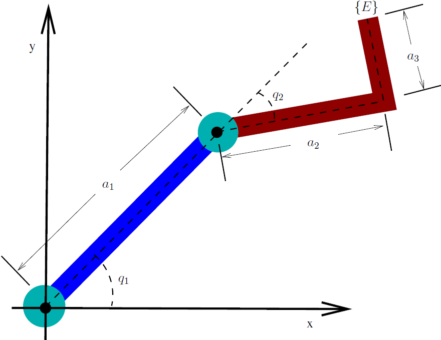
Consider the following two link robot where the second link has a 90 degree bend. The lengths of links are shown in the MATLAB code below. We want to find the joint angles $q_1$ and $q_2$ so that the end effector $\{E\}$ is at position (2, 3.2).

The MATLAB script below shows both a closed form solution and also uses a numeric algorithm to find a solution. Finding the closed form solution was largely interactive with MATLAB.

global a1  a2 a3;
a1 = 2; a2 = 1.5; a3 = 1;
% The above constants should not be changed. Otherwise, some of the numbers
% in the program will not be correct. Note: If the variables (a1, a2,
% and a3) are kept as variables, then the closed form equations become
% very messy. So we will consider this as a fixed dimension robot.

E = [2; 3.2];  % Target end effector position

%% Reachability   NOTE: When developing an inverse kinematic solution,
%                       do reachability after working out the
%                       inverse kinematic equations.
%
% If the target position is out side the robot's reach, then no
% solution is available. From the geometry of the robot, the reach of the
% robot is the length of the first arm (+-) the distance from the start
% to end of the second arm.
% c = norm([a2; a3]);
% minReach = a1 - c;
% maxReach = a1 + c;
%
% Check if the robot can reach the desired position
n = norm(E);
if n < 0.2 || n > 3.8
    disp('The desired end effector position is not reachable');
    return;
end
fprintf('Desired position: %f %f\n', E(1), E(2));

%% Closed form solution
%
% Use the Symbolic Math Toolbox interactively to find equations
% for joint angles.
%
% syms q1 q2;
% T = trchain2('R(q1) Tx(a1) R(q2) Tx(a2) Ty(a3)', [q1 q2]);
% x = T(1,3);
% y = T(2,3);
% % % --- x and y have some sin and cos terms of the same angles
% % % try x^2 + y^2, which is E'*E (dot product with self)
% % %
% simplify(x^2 + y^2)
% % ans =
% % 6*cos(q2) - 4*sin(q2) + 29/4
% This is of the form a*cos(q2) + b*sin(q2) = c

% This is of the form a*cos(q2) + b*sin(q2) = c
q2 = get_angle(6, -4, (E'*E - 29/4));
q2 = min(q2);             % elbow up

%%
% Now for q1. We have one unknown (q1) and two equations
% (x == E(1), and y == E(2)). However, both equations use q1 as
% sin(q1) and cos(q1) functions.  So we can use both equations
% to find cos(q1) and sin(q1) as a system of equations.
% Then use an inverse tanget function to get q1.

% First get numeric values for q2 terms.
C2 = cos(q2);
S2 = sin(q2);

% Symbolic math for finding the equations
%
% syms q1 q2;
% T = trchain2('R(q1) Tx(a1) R(q2) Tx(a2) Ty(a3)', [q1 q2]);
% x = T(1,3);
% y = T(2,3);
%    Find and rearrange x and y in terms of C2 and S2
% x = (2 + 3*C2/2 - S2)*cos(q1) - (C2 + 3*S2/2)*sin(q1)  == E(1)
% y = (C2 + 1.5*S2)*cos(q1) + (2 + 1.5*C2 - S2)*sin(q1) == E(2)
A = [(2 + 3*C2/2 - S2) -(C2 + 3*S2/2);
    (C2 + 1.5*S2) (2 + 1.5*C2 - S2)];
Q1 = A\E;         % Q1 is now vector [cos(q1); sin(q1)]
q1 = atan2(Q1(2), Q1(1));

fwd = fwd_kin([q1 q2]);
fprintf('Closed form 2:\n\tjoint angles: %f %f\n', q1, q2);
fprintf('\tposition = %f %f\n', fwd(1), fwd(2));

%% Numerical solution -- for comparison and example only
% Now, use numerical methods to solve the inverse kinematics problem

fun = @(q) norm(fwd_kin(q) - E);
Q = fminsearch(fun, [pi/4 -pi/4]);
fprintf('Numeric:\n\tjoint angles: %f %f\n', Q(1), Q(2));
E1 = fwd_kin(Q);
fprintf('\tposition: %f %f\n', E1(1), E1(2));

%% Plot it
T = trot2(q1)*transl2(a1,0);
p1 = T(1:2,3);
T = trot2(q1)*transl2(a1,0)*trot2(q2)*transl2(a2,0);
p2 = T(1:2,3);
T = trot2(q1)*transl2(a1,0)*trot2(q2)*transl2(a2,a3);
p3 = T(1:2,3);
figure, hold on
plot([0 p1(1)], [0 p1(2)], 'LineWidth', 3);
plot([p1(1) p2(1) p3(1)], [p1(2) p2(2) p3(2)], 'LineWidth', 3);
grid on
daspect([1 1 1])
title('Plot of Robot Arm');
hold off

%% Helper private functions
% solution to a*cos(theta) + b*sin(theta) = c
function theta = get_angle(a, b, c)
    theta = zeros(1,2);
    d = sqrt(a^2 + b^2 - c^2);
    e = atan2(a,b);
    theta(1) = atan2(c,d) - e;
    theta(2) = atan2(c,-d) - e;
    theta = wrapToPi(theta);
end

% The forward kinematics as a private function to the script
function p = fwd_kin(q)
    global a1  a2 a3;
    T = trot2(q(1))*transl2(a1,0)*trot2(q(2))*transl2(a2, a3);
    p = T(1:2,3);
end

4.1.2. Inverse Kinematics¶

4.1.2.1. Solving Inverse Kinematics Problems¶

4.1.2.2. Inverse Kinematic Example¶

Table of Contents

Previous topic

Next topic

This Page