3.1.1. Rotation of a Point
See also
This YouTube Video by Peter Corke discusses rotation of points.
Rotation is a very important topic to both machine vision and robotics. Pixels in an image might be rotated to align objects with a model. After describing rotation of a point, we can extend the concept of a rotation matrix to transformations consisting of rotation and translation. Then we consider transformations of coordinate frames that are used to describe the pose of robots and robotics moving parts.
Here, we only consider rotating points about the origin. Rotation about other points is an extension of rotating about the origin.
Point  is rotated by an angle
  about the
origin to point
about the
origin to point  .
.
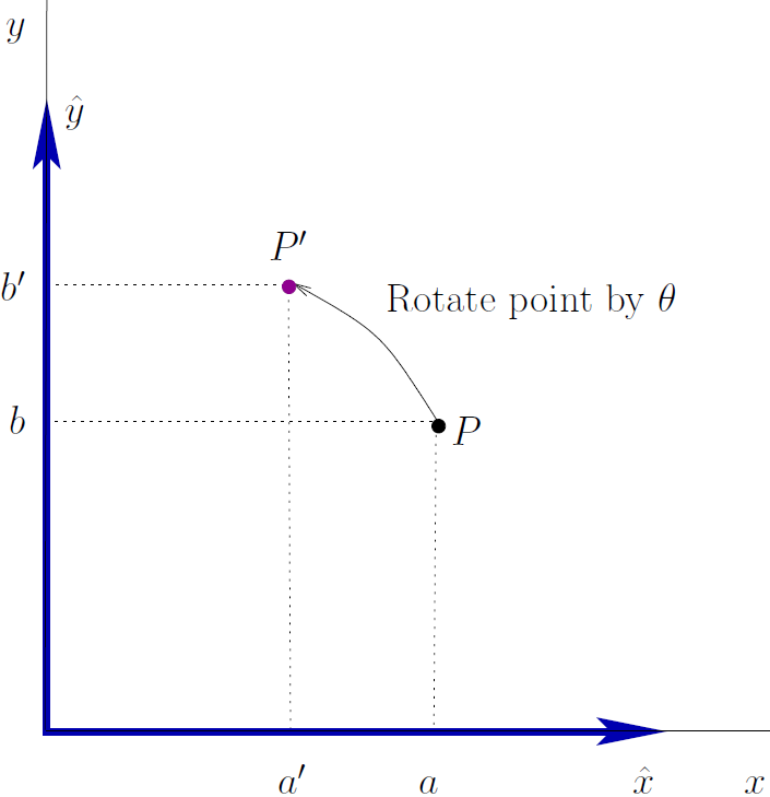
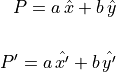
To facilitate the discussion, the point  is defined in terms of
unit vectors
is defined in terms of
unit vectors  and
and  . The new
location,
. The new
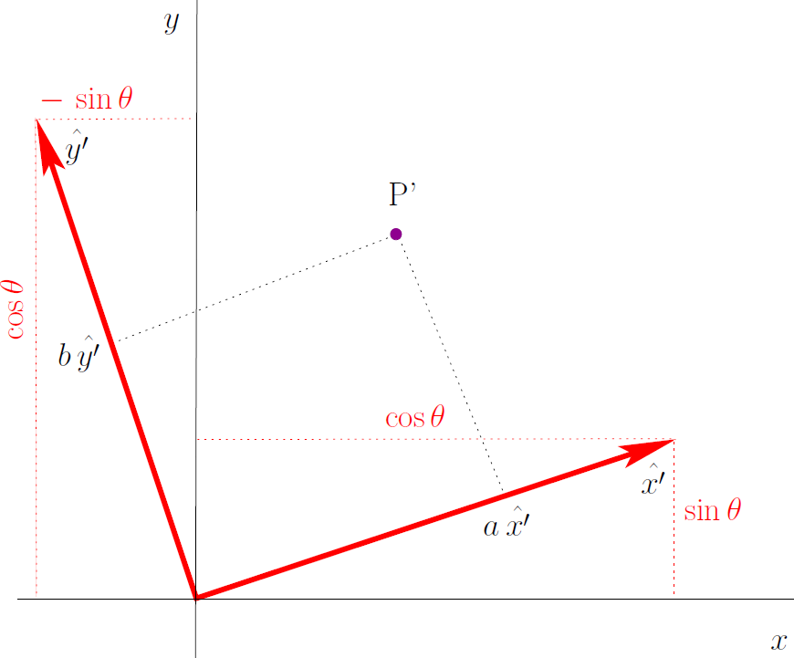
location,  is then defined by unit vectors
  and
and
 formed by rotating
  and
and  by
the angle .
by
the angle .
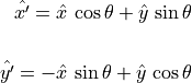

Expressed in matrix notation:
![\begin{array}{ll}
P' &= \spalignmat{\hat{x}, \hat{y}}
\spalignmat[r]{\cos\theta, -\sin\theta;
\sin\theta, \cos\theta}
\spalignvector{a; b} \\ \\
&= \spalignmat{1, 0; 0, 1}
\spalignmat[r]{\cos\theta, -\sin\theta;
\sin\theta, \cos\theta}
\spalignvector{a; b} \\ \\
&= \spalignmat[r]{\cos\theta, -\sin\theta;
\sin\theta, \cos\theta}
\spalignvector{a; b}
\end{array}](../_images/math/c61177bd3b5627e5a6e5332314a88061a34b9a07.png)
Thus, we have a 2-by-2 rotation matrix, which when multiplied by a vector specifying an original location of the point yields the coordinates of the rotated point.
![R(\theta) = \spalignmat[r]{\cos\theta, -\sin\theta;
\sin\theta, \cos\theta}](../_images/math/226b16a38a61b064424c54078d5e7411c8155367.png)
The rotation matrix has the following special properties.
The columns define unit vectors for the rotated coordinate frame.
The sum of each column is one.
The columns are orthogonal. The dot product of the columns is zero. It is called an orthonormal matrix.
 .
.The determinant,
 , thus it
is never singular.
, thus it
is never singular.
3.1.2. Homogeneous Matrix
Geometric translation is often added to the rotation matrix to make a matrix
that is called the homogeneous transformation matrix. The
translation coordinates ( and
and  ) are added in a third
column. So that the resulting matrix is square, an additional row is also
added.
) are added in a third
column. So that the resulting matrix is square, an additional row is also
added.
![T(\theta, x_t, y_t) = \spalignmat[r]{\cos\theta, -\sin\theta, x_t;
\sin\theta, \cos\theta, y_t;
0, 0, 1}](../_images/math/45f29291fc78c24fe9597a37ef4f834b23815cc7.png)
Homogeneous rotation alone is given by the matrix.
![R(\theta) = \spalignmat[r]{\cos\theta, -\sin\theta, 0;
\sin\theta, \cos\theta, 0;
0, 0, 1}](../_images/math/178f7622f99b9fd387cd7c3321ac4a2426146e74.png)
Homogeneous translation alone is given by the matrix.
![T_t(x_t, y_t) = \spalignmat[r]{1, 0, x_t; 0, 1, y_t; 0, 0, 1}](../_images/math/95ed4a891c7f9b696170fee0627b2bedac4ee438.png)
The combined rotation and translation homogeneous transformation matrix can be found by matrix multiplication.

Note
The inverse of the homogeneous matrix is not as simple to compute as it is for the rotation matrix, where is the inverse is found by simply taking the transpose of the matrix.
3.1.2.1. Applying Transformations to a Point
When applied to a point, the homogeneous transformation matrix defines rotation followed by translation in the original coordinate frame. It is not translation followed by rotation. It is also not rotation defining a new coordinate frame, followed by translation in the new coordinate frame. The following MATLAB session demonstrates this.
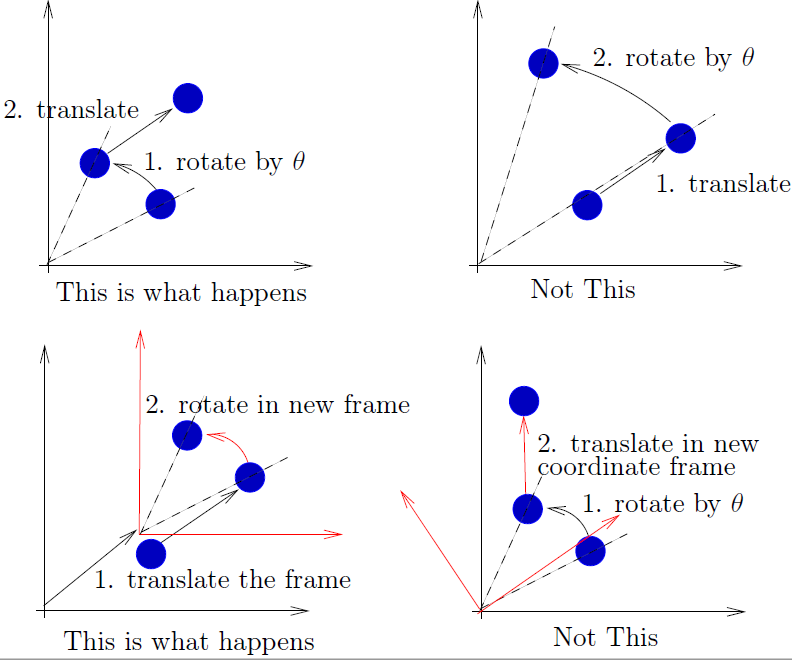
Fig. 3.1 A transformation applied to a point,  , rotates and
translates the point relative to the original coordinate frame.
, rotates and
translates the point relative to the original coordinate frame.
Note that although the variables shown here are simple vectors and matrices, which are not difficult to deal with directly in MATLAB, some utilities from Peter Corke’s Robotics Toolbox are used. An object of type SE2 provides a simple way to apply homogeneous transforms.
>> % Define a point at (1, 1)
>> P = [1;1];

>> % Define a transformation, rotation (pi/3) and translation (2, 1)
>> T = SE2(2, 1, pi/3)
T =
    0.5000   -0.8660    2.0000
    0.8660    0.5000    1.0000
         0         0    1.0000

>> % Apply the transform direct to P using the SE2 object
>> % The SE2 object shows the result in Euclidean coordinates
>> T*P
ans =
    1.6340
    2.3660

>> % get the transform matrix, rotation, and translation from T
>> Tm = T.T
Tm =
    0.5000   -0.8660    2.0000
    0.8660    0.5000    1.0000
         0         0    1.0000
>> R = T.R
R =
    0.5000   -0.8660
    0.8660    0.5000
>> t = T.t
t =
    2
    1

>> % transformation of P using the transfom matrix.
>> % Note that [P;1] is point P in homogeneous coordinates
>> % h2e returns Euclidean coordinates from homogeneous
>> h2e(Tm*[P;1])
ans =
    1.6340
    2.3660

>> % Here we use the rotation matrix and translation vector directly,
>> % to show difference in transform order.

>> % rotate, then translate - same result as T*P
>> R*P + t
ans =
    1.6340
    2.3660

>> % translate then rotate is different
>> R*(P + t)
ans =
   -0.2321
    3.5981
3.1.2.2. Homogeneous Transformation
Warning
Watch the subtle details here.
In the previous example, we showed applying the translation by adding the translation vector to the point vector. That is because we kept the coordinate frame constant. Just as rotation can be expressed with a homogeneous matrix, so can translation. We then multiply matrices to show translation.
We can also find the homogeneous matrix for translation and rotation by multiplication, but the order of the multiplication may be different than you expect because the coordinate frame changes with rotation.
Coordinate frames are different than points in that when we rotate a coordinate frame, the origin of the frame stays in the same position relative to the world frame. Rotation of a coordinate frame always changes the frame used for future translations. Thus, we think of transformation of a coordinate frame as translation in the original frame followed by rotation – opposite of points.
% translation alone
>> Tx = transl2(2, 1)
Tx =
    1     0     2
    0     1     1
    0     0     1

% apply translation to a point with homogeneous coordinates
>> P = [1 1 1]'
P =
    1
    1
    1
>> Tx*P   % homogeneuos
ans =
    3
    2
    1

% rotation alone
>> Tr = SE2(0, 0, pi/3).T
Tr =
    0.5000   -0.8660         0
    0.8660    0.5000         0
         0         0    1.0000

% apply rotation to a point
>> Tr*P
ans =
   -0.3660
    1.3660
    1.0000

% find the combined tranformation, same as previous T.
% translation before rotation
>> Tx*Tr
ans =
    0.5000   -0.8660    2.0000
    0.8660    0.5000    1.0000
         0         0    1.0000

% the following does the translation in a rotated coordinate frame,
% rotation before translation is different than T -- wrong answer.
>> Tr*Tx
ans =
    0.5000   -0.8660    0.1340
    0.8660    0.5000    2.2321
         0         0    1.0000
Note that multiplication of transformation matrices is NOT commutative. The order in which the matrices are multiplied matters to the final result.
The last example shows what happens when the coordinate frame is changed, which relates to the next topic.