4.5. Generating Random Numbers
Random numbers are useful for creating simulations and emulating the presence of noise or random chance. MATLAB includes continuous and discrete random number generators for uniform and normal distributions. Random number generators for different probability distributions can be derived from the uniform and normal generators. Exponential Random Number Generator lists a short function to generate random numbers according to the exponential probability distribution. The Statistics and Machine Learning Toolbox has random number generators for other distributions. A search on the Internet will also find the source code for random number generators for other distributions.
- rng
The
rngfunction seeds MATLAB’s random number generating functions to generate either a repeatable or unique sequence of pseudo-random numbers. Seeding the random number generator with a fixed number results in the same sequence of numbers, which is helpful for comparisons of algorithms, and is a debugging strategy because the outcome is reproducible. Userng("shuffle")to get a unique sequence of numbers. Theshuffleoption sets the seed from the current time.
- rand
The
rand(n)function creates an \(n{\times}n\) matrix of uniformly distributed random numbers in the interval (0 to 1).rand(m, n)creates a \(m{\times}n\) matrix or vector. To generate \(n\) random numbers in the interval \((a, b)\) use the formular = a + (b-a)*rand(1, n).
- randn
The
randnfunction creates random numbers with a normal (Gaussian) distribution. The parameters torandnregarding the size of the returned data are the same as forrand. The values returned fromrandnhas a mean of zero and a variance of one. To generate data with a mean of \(a\) and standard deviation of \(b\), use the equationy = a + b*randn(N,1).
- randi
The
randi(Max, m, n)function creates a \(m{\times}n\) matrix of uniformly distributed random integers between 1 and a maximum value. Provide the maximum value as the first input, followed by the array size.
- randperm
The
randpermi(n)function returns a row vector containing a random permutation of the integers from 1 to n without repeating elements. One application of this is to achieve a shuffle operation, like with a deck of playing cards. Similarly,randperm(n,k)returns a row vector containing k unique integers selected randomly from 1 to n.
Usage code and histograms of each random number generator are shown in RandGensPlots.m and Fig. 4.8.
% File: randGenPlots.m
t = tiledlayout(3, 1);
title(t, 'Random Number Generators')
nexttile;
histogram(20*rand(1, 1000), 40)
title('rand \sim U(0, 20)')
nexttile;
histogram(randi(20, 1, 1000), 20)
title('randi \sim U(1, 20) integers')
nexttile;
histogram(10 + 3*randn(1, 1000), 40)
title('randn \sim N(10, 3)')
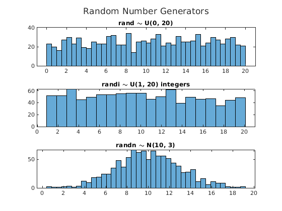
Fig. 4.8 Histograms from random number generators
4.5.1. Exponential Random Number Generator
Recall from Continuous Distributions that equation (4.2) is the CDF of the exponential probability distribution.
Equation (4.3) shows the inverse of the CDF found by
letting \(y = F(a)\) and solving for \(a\). The randexp
function in randexp generates random numbers with an
exponential distribution using equation (4.3) and the
rand function that gives a uniform distribution in the interval
\((0, 1)\).
Fig. 4.9 shows a histogram of a random variable
created with our random number generator.
function X = randexp(lambda, m, n)
% RANDEXP - Simple exponential distribution random
%    number generator. If you have the Statistics
%    and Machine Learning Toolbox, use exprnd.
%
% lambda - exponential distribution parameter
%   mean(X) ~ 1/lambda, var(X) ~ 1/lambda^2
%   Output is size m x n
    y = rand(m, n);      % y ~ U(0, 1)
    y(y == 1) = 1 - eps; % protect from divide by 0
    X = log(1./(1-y))./lambda; % inverse of CDF
end
>> X = randexp(2.0, 1, 500);
>> x_bar = mean(X)
x_bar =
    0.5005
>> s2 = var(X)
s2 =
    0.2887
>> histogram(X)
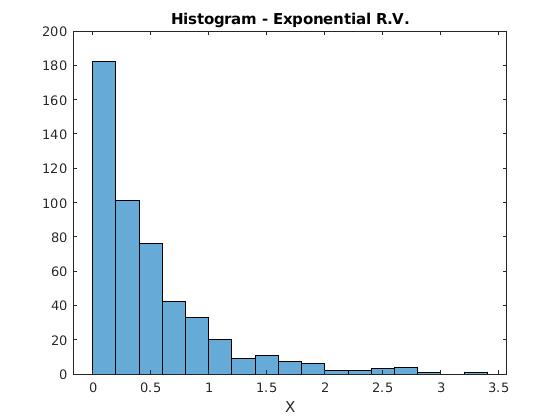
Fig. 4.9 Histogram from the exponential random number generator.
4.5.2. Monte Carlo Simulation
Here is a fun application of a random number generator. The script in
randpi performs what is called a Monte Carlo simulation to
estimate the value of \(\pi\) [GUTTAG16]. We
create a set of uniformly distributed random points in a square between
\(-1\) and \(1\) in both the \(x\) and \(y\) directions.
Then we relate the ratio of the number of points that fall inside a
circle of radius 1 to the total number of points. The number of points
inside the circle should be related to the area of the circle. Since the
lengths of the sides of the square are 2, the area of the square is 4,
while the area of the unit circle is \(\pi\). A plot of the points
inside and outside the circle is shown in Fig. 4.10.
% File: randpi.m
% Script to use a random number generator to estimate the
% value of PI using a Monte Carlo simulation.

N = 1000000;

% 2-D points on a plane, uniform distribution in each
% dimension between -1 and 1.
points = 2*rand(2, N) - ones(2, N);
% scatter(samples(1,:), samples(2,:), '.')
radii = vecnorm(points);  % distance of each point from (0, 0).
inCircle = radii <= 1;    % points inside circle

% Area of square is 4. Area of circle is pi. So the ratio
% of points inside the circle to the total should be pi/4.
piEstimate = 4*nnz(inCircle)/N;
error = 100*abs(piEstimate - pi)/pi;
disp(['Estimate of pi is: ', num2str(piEstimate)])
disp(['The error was ', num2str(error), ' percent.'])

% plot the points inside and outside of the circle.
figure, axis equal
hold on
scatter(points(1, inCircle), points(2, inCircle), '.')
scatter(points(1, ~inCircle), points(2, ~inCircle), '.')
hold off
title('Monte Carlo Estimate of \pi')
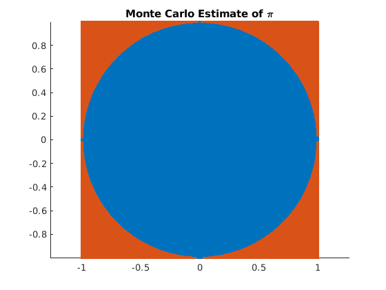
Fig. 4.10 The ratio of points inside the circle to total points is close to \(\pi/4\).
4.5.3. Random Casino Walk
Another use of random number generators is a random walk simulation. Random walks represent a cumulative series of random numbers that, at each step, can move the state of the simulation. Random walks can be performed in different dimensions. In the example here, the dimension of the random walk is one.
Following is a simulation script for playing slot machines at a casino. One hundred players each start with 80 quarters ($20). Each player plays all 80 quarters and counts their winnings at the end. The machines are programmed to return 80% of what they take in. So the expected winnings of each player are $16 after spending $20 (loss of $4). Sometimes the machines give winners 4 quarters, and sometimes they payout 8 quarters. Logical arrays simplify the implementation. We use integer random numbers with a uniform distribution for events with simple percentages of occurrence. A histogram of the winnings for the 100 players is shown in Fig. 4.11. The shape of the histogram also affirms the central limit theorem described in Central Limit Theorem.
% File: casinoWalk.m
% Random walk simulation of playing slot machines.
% 100 people each start with 80 quarters ($20).
% They play all 80 quarters and see how much money they
% have in winnings. The slot machines payout 80% of
% what they take in. Half of the time, they use 1/5 odds
% to pay 4 quarters. The other times, they use 1/10 odds
% to pay 8 quarters. You should find the average winning
% to be about -4 dollars.

winning = zeros(1, 100);
for p = 1:100   % for each player
    oneIn10 = randi(2, 1, 80) == 2; % win 1/10 or 1/5
    rand = randi(10, 1, 80);
    payout = zeros(1, 80);
    payout(oneIn10 & rand == 10) = 8;
    payout(~oneIn10 & rand > 8) = 4;
    winning(p) = sum(payout)/4 - 20; % net winnings
end
disp(['Average winning = $', num2str(mean(winning))])
histogram(winning, 25)
xlabel('Winnings ($)')
ylabel('Players out of 100')
title('Slot Machine Net Winnings on $20')
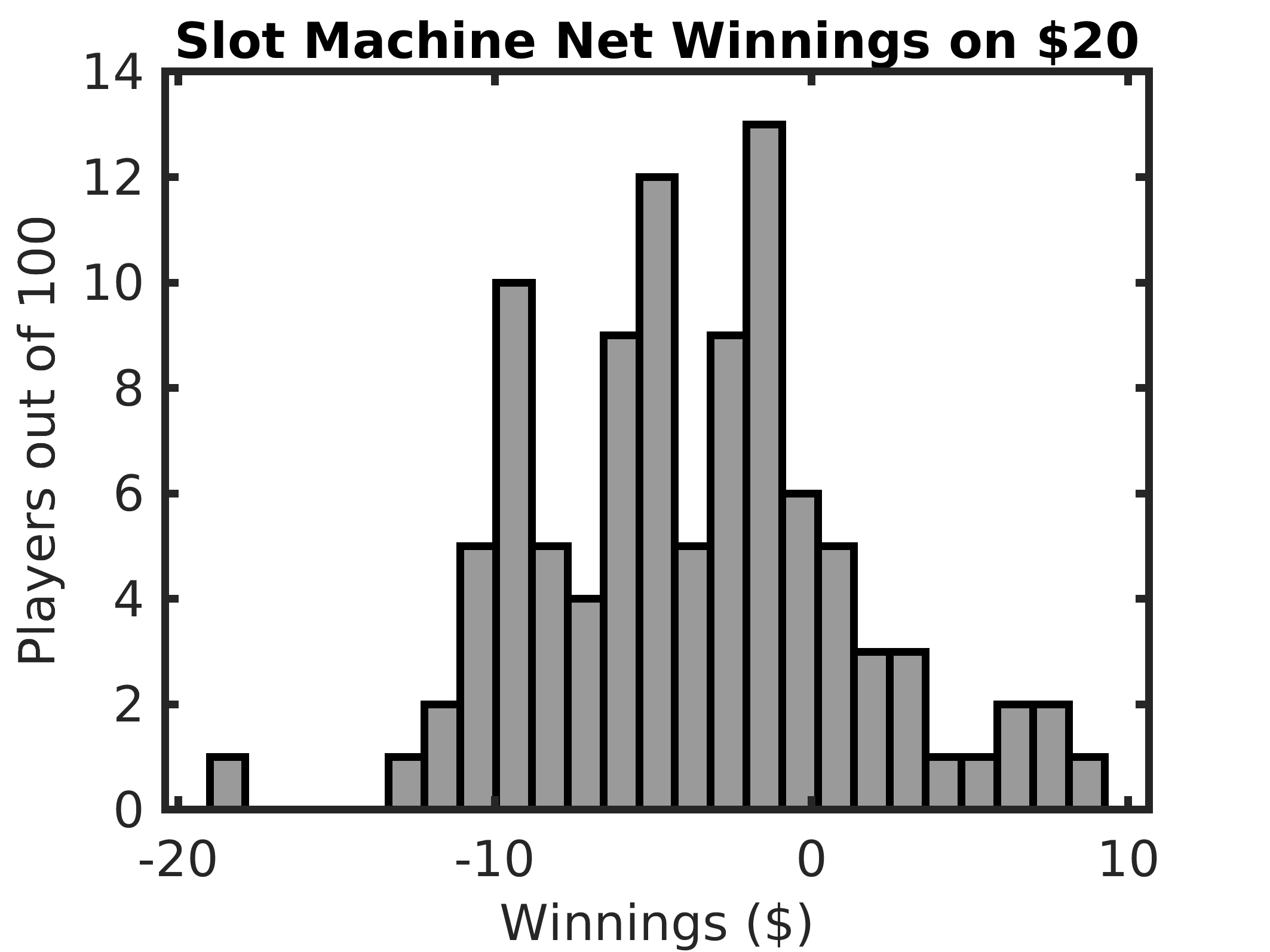
Fig. 4.11 Histogram of winnings after spending $20 on slot machines.
