17.8. Frequency Domain Filters
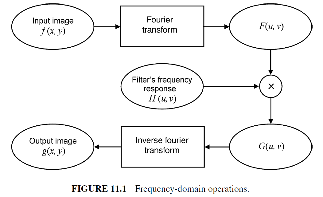
Whereas convolution is used to evaluate filters in the spatial domain, filtering is implemented in the frequency domain by multiplication. The image in the frequency domain is multiplied by the filter’s frequency response in the frequency domain. Thus, the filter transfer function is simply a matrix of the same size as the image. The complex values of the image in the frequency domain are simply multiplied element by element with the filter transfer function to amplify or attenuate specific frequencies of the image. The inverse Fourier transform is then used to generate the output image.
For each filtering operation, we will describe the construction three types of filters in the frequency domain.
-
ideal filters Ideal filters are quick and easy to implement and give an easy to understand appreciation of the filter. Unfortunately, ideal filters typically yield undesired results. Specifically, ideal filters suffer from a problem known as ringing where extra lines appear around the edges of objects in an image. (see What Causes Ringing?)
-
Gaussian filters The shape of a Gaussian filter transfer function is that of the bell-shaped curve that models the probability distribution function of a normal or Gaussian stochastic process. The smooth transition between the pass-band and stop-band produces good results with no noticeable ringing artifacts. The cutoff frequency of Gaussian filters is determined by a variable (
 ).
).
-
Butterworth filters The shape of a Butterworth filter transfer function is tunable. The order of the filter (
 ) determines the steepness of the transition
between the pass-band and stop-band. It can assume a gentle transition
like that seen in Gaussian filters, or it can assume an abrupt transition
like ideal filters. A nice aspect of Butterworth filters is that the
cutoff frequency is a parameter of transfer function equation. Thus, it
is simpler to determine the parameters from examining the image in the
frequency domain.
) determines the steepness of the transition
between the pass-band and stop-band. It can assume a gentle transition
like that seen in Gaussian filters, or it can assume an abrupt transition
like ideal filters. A nice aspect of Butterworth filters is that the
cutoff frequency is a parameter of transfer function equation. Thus, it
is simpler to determine the parameters from examining the image in the
frequency domain.
17.8.1. Filter Parameters
-
Distance Function To generate filter transfer functions, it is necessary to know the distance of each element of the transfer function to the origin (0,0). In the filter transfer function equations, this distance to the origin is denoted as
 , or simply as
  . Since the
frequency domain data ranges from
. Since the
frequency domain data ranges from  to
to  in
both the horizontal and vertical direction, rather than between
in
both the horizontal and vertical direction, rather than between
 and
and  ), it is convenient to use a special
function to calculate the distances. A function to build a matrix of
these distances is included with the MATLAB code for completing the
tutorials.
), it is convenient to use a special
function to calculate the distances. A function to build a matrix of
these distances is included with the MATLAB code for completing the
tutorials.
-
Cutoff Frequency The transition point between the pass and stop bands of the filter is denoted as
 .
.
-
Band Width For band-reject and band-pass filters, where the data between lower and upper cutoff frequencies is either rejected or passed, the width is denoted as
 .
.
17.8.2. Low-Pass Filters
Low pass filters remove higher frequencies, thus blurring some image content.
-
ideal low-pass filter 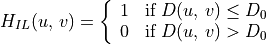
-
Gaussian low-pass filter 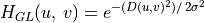
-
Butterworth low-pass filter ![H_{BL}(u,\,v) = \frac{1}{1 + \left[ D(u,v)/\,D_0 \right]^{2n}}](../_images/math/e17d8ec7ea863a4af6f391534602f1d6b7d29972.png)
17.8.3. High-Pass Filters
The concept of high-pass filtering is to remove lower frequency content while keeping higher frequencies. With image processing, this, by it self, yields undesirable results. Particularly, removing the overall brightness represented at position (0, 0) of the image in the frequency domain is not desired. Thus, to preserve the low-frequency content while emphasising the high-frequency content we alter the transfer function with a high-frequency emphasis equation.

A value of one for both  and
and  is common.
-
ideal high-pass filter 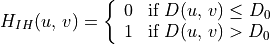
-
Gaussian high-pass filter 
-
Butterworth high-pass filter ![H_{BH}(u,\,v) = \frac{1}{1 + \left[ D_0/\,D(u,v) \right]^{2n}}](../_images/math/99d922f5bcd690bd9055012030cdfcfab46e6e35.png)
17.8.4. Band-reject Filters
Band-reject and Band-Pass filters are used less in image processing than low-pass and high-pass filters.
Band-reject filters (also called band-stop filters) suppress frequency
content within a range between a lower and higher cutoff frequency. The
parameter here is the center frequency of the reject band.
-
ideal band-reject filter 
-
Gaussian band-reject filter 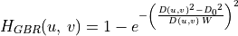
-
Butterworth band-reject filter ![H_{BBR}(u,\,v) = \frac{1}{1 + \left[\frac{D(u,v)\,W}
{D(u,v)^2 - {D_0}^2} \right]^{2n}}](../_images/math/1490cb8288244011390f9c0dc4d617b81fff4d92.png)
17.8.5. Band-Pass Filters
A band-pass filter is the opposite of a band-reject filter. It only passes frequency content within a range. A band-pass filter is obtained from a band-reject filter as: