9. Color Images
Reading Assignment
Please read section 10.2.4-10.2.6, 10.3.6 of [RVC] and browse through chapter 16 of [PIVP].
Video Resources

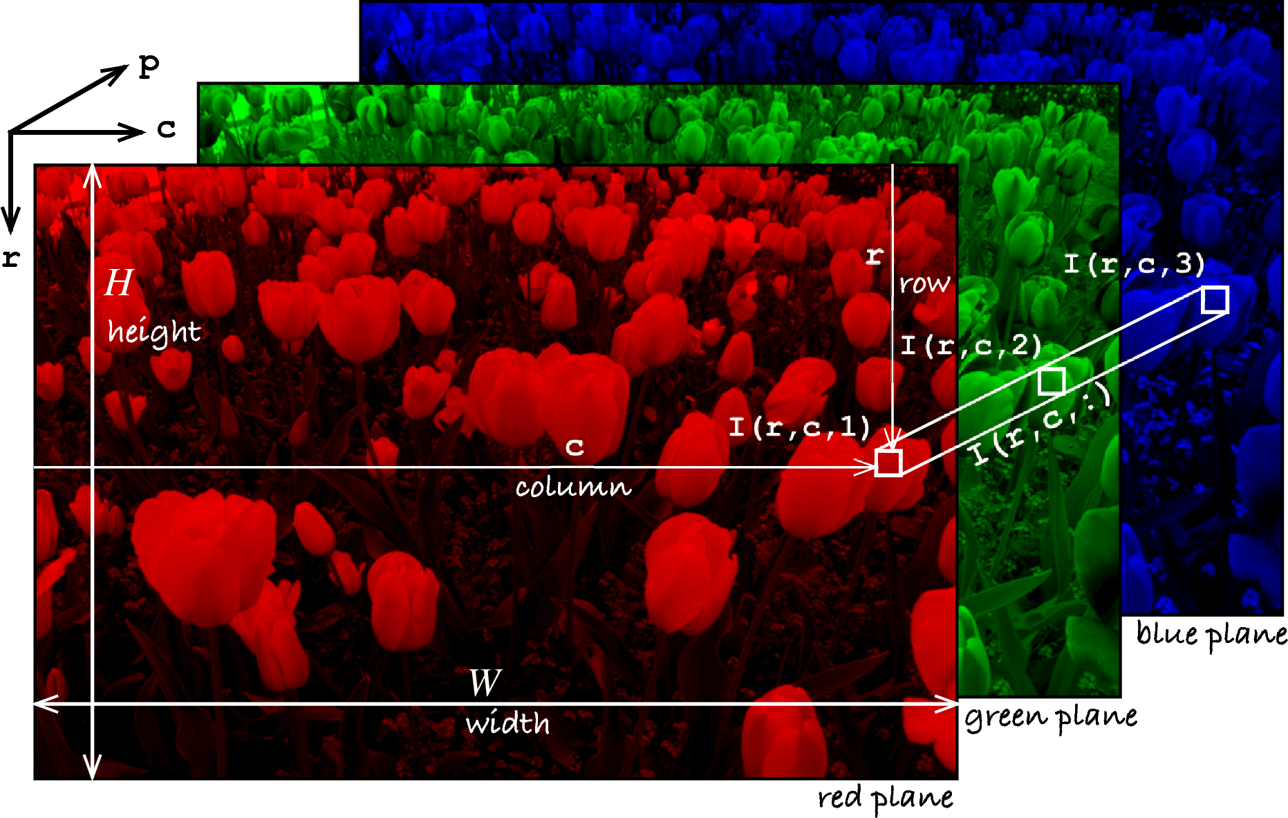
Figure 12.2 from [RVC]. Color images are made of three monochrome image for each red, green, and blue.
9.1. Chromaticity Coordinates
When working with gray-scale images, we consider the intensity, or
brightness, of the pixels. But to distinguish between different colors,
regardless of their intensity, we want to transform the RGB values into
chromaticity coordinates and we divide the RGB values by the sum, by the
total tristimulus, we end up with these variables, little  ,
little
  and little
  .
.

These values vary between zero and one and
sum to one. Therefore, one of the coordinates is redundant and typically we
consider just the little  and little
  values.
The following code produces a chromaticity diagram.
% Chromaticity Diagram
N = 200;
[Red, Green] = meshgrid(linspace(0,1,N), linspace(0,1,N));
notValid = (Red + Green) > 1;
Red(notValid) = 0;
Green(notValid) = 0;
Blue = ones(N) - Red - Green;
Blue(notValid) = 0;
color_chart = zeros(N,N,3);
color_chart(:,:,1) = Red;
color_chart(:,:,2) = Green;
color_chart(:,:,3) = Blue;
idisp(flipud(color_chart), 'nogui');
The following example from Peter Corke demonstrates forming a logical image by distinguishing color.
Load the image tomato_124.jpg as type double and display.
>> im = iread('tomato_124.jpg', 'double');
>> idisp(im)
We can perform gamma correction when loading the image by supplying additional arguments. Display the result.
>> im = iread('tomato_124.jpg', 'double', 'gamma', 2.2);
>> idisp(im)
We can view the individual color planes. Let’s look at the red plane. The tomato fruit are quite bright here.
>> idisp(im(:,:,1))
And the green plane where the tomato fruit are quite dark.
>> idisp(im(:,:,2))
Extract each of the color planes into separate matrices and calculate the luminance image by summing these matrices. Display the luminence image.
>> R = im(:,:,1);
>> G = im(:,:,2);
>> B = im(:,:,3);
>> Y = R + G + B;
>> idisp(Y)
This luminance image can be used to calculate the chromaticity coordinates using the element-wise division operator (./). Display these chromaticity channels.
>> r = R ./ Y;
>> g = G ./ Y;
>> idisp(r)

>> figure(2)
>> idisp(g)
We can attempt to extract the tomato fruit in the image by performing thresholding and logical operations on the red and green chromaticity channels. Display this binary image.
>> tom = (r > 0.8 & g < 0.2);
9.2. HSV Colorspace
Another popular representation of color comes from the HSV colorspace. Like
RGB, three planes describe a color picture. The H (first) plane describes the
color of each pixel. The H value has a range from 0 to 1 that corresponds to
the color’s position on a color wheel. As the hue increases from 0 to 1, the
color transitions from red to orange, yellow, green, cyan, blue, magenta, and
finally back to red. You may find resources on the Internet describing the H
values as between 0 to 360 degrees, where one can simply divide by 360 to get
the scale used by MATLAB. MATLAB has functions rgb2hsv() and hsv2rgb()
for converting images between the two color systems.
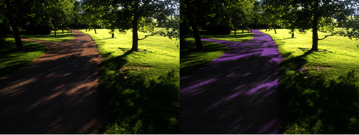
Find a picture you like, maybe of a car, house, motorcycle, or similar and try to change the color of parts of the image. For example, I changed the color of the sidewalk in this image from a park to a K-State purple color. Hint, you will need to use a logical vector mask to identify the pixels of interest.

