15. Edge Detection
Video Resources
Peter Corke Finding Line Features.
This topic is of special interest to machine vision inspection systems. We wish to identify edges on objects in an image. In particular, we would also like to find shapes such as lines or circles along the edges.
Finding pixels that are on an edge is a matter of applying first and second derivatives to an image, mostly through the use of special spatial filters (see Neighborhood (Spatial) Processing). We will look through the author slides from chapter 14 of [PIVP] and complete an abbreviated tutorial.
After finding edge pixels, the Hough Transform can be used to find edge features. The Hough Transform can be a bit tricky at first to understand. Dr. Corke’s video (link above) does a nice job of explaining it and I’ll go over it from the notes below and the tutorial.
15.1. Hough Transform
After other algorithms have been used to identify edge pixels in an image, the Hough transform may be used to associate a math equation (for later use) to some shapes outlined by the edges. The Hough transform can be used to find lines, circles and ellipses. Here, we only examine its use to find lines.
The Hough transform uses voting to estimate the parameters of line equations from pixels identified as edges. Votes will be cast for lines that do not exist, but when the pixels are aligned in the form of lines then the true lines will receive the most votes.
15.1.1. Line Equations
The most common equation for a line is the slope, intercept form:

The value of  represents the slope of the line and
  is the
value where the line intercepts the y axis.
is the
value where the line intercepts the y axis.
The Hough transform uses the normal form line equation to identify the parameters of the line equation.
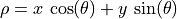
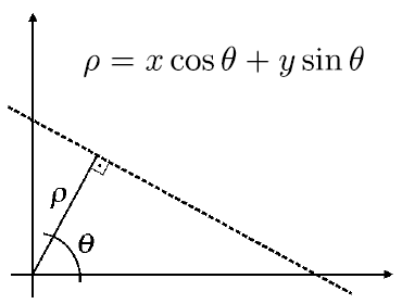
In the normal form line equation,  and
and  describe the length and angle of a line from the origin and perpendicular
to the line of interest.
describe the length and angle of a line from the origin and perpendicular
to the line of interest.
For each edge pixel in the image, a curve is formed from the normal form
equation for a set of angles () between  and
and
 . Each point of the curve represents the and
describing one line that might go through the edge pixel.
Each point of the curve is counted as belonging to a regional bin of
and values. The bins with the most votes are
used to describe lines in the image.
. Each point of the curve represents the and
describing one line that might go through the edge pixel.
Each point of the curve is counted as belonging to a regional bin of
and values. The bins with the most votes are
used to describe lines in the image.
Note that for some lines, the value of may be negative.
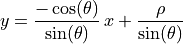
Given a and , the normal form equation can be
used to describe a line in slope, intercept form.
15.1.1.1. Example
MATLAB’s IPT includes functions that take most of the work out of applying the Hough transform, but the following manual demonstration illustrates how the transform finds line equations.
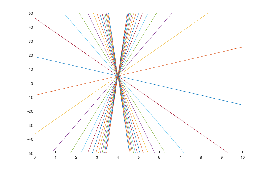
Consider the line 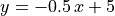 . In the following MATLAB code, we
plot lines for integer points on the line,
. In the following MATLAB code, we
plot lines for integer points on the line,  .
.
theta = linspace(-pi/2, pi/2);
figure
xlabel('\theta'), ylabel('\rho');
hold on
for x = 0:5
    y = -0.5*x + 5;
    plot(theta,(x*cos(theta) + y*sin(theta)));
end
hold off
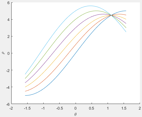
From examining the graph, the point where the curves intersect is
approximately,  ,
,  . Applying these
values to our line equation yields an equation close to our original line
equation (with some error).
. Applying these
values to our line equation yields an equation close to our original line
equation (with some error).
15.1.2. Applying the Hough Transform
First, find edge pixels of an image. We will consider each pixel as possibly being a point on a line. Since we don’t know the equation for the line, or if the edge point is part of a line, we will evaluate a set of possible lines going through this point.
We cast a vote for each possible and for the
point. If other pixels are also points on a line, then the and
for the line will get a lot of votes.
Create a 2D array corresponding to a discrete set of values for
and . Each element in this array is often referred to as
an accumulator cell.For each edge pixel
 in the image and for each chosen value
of , compute
in the image and for each chosen value
of , compute 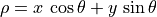 and write the result in the corresponding position
  in the accumulator array.
The highest values in the
array will correspond to
the most relevant lines in the image.Finally, determine the line equations: