4.9. Sampling and Confidence Intervals

As mentioned in Introduction to Statistics, it is challenging to determine statistics for a large population. Each sample set will likely have a different mean when sampling a large population. However, we can calculate a range of values for which we have confidence that the actual population mean is within. The central limit theorem and the standard normal distribution give us the tools to do this. In particular, we will use the \(Z\) variable defined in equation (4.4).

From the CDF of a standard normal distribution, we can establish probabilities and introduce \(Z\)-critical values, which are used to find an interval where we have confidence at a level of \(C\) that the actual population mean is within the interval [HOGG78]. We can use the \(Z\)-critical values to test if a sample likely came from the same population or perhaps is from a different population. The \(Z\)-critical values for establishing confidence levels are shown in table Z–critical values. A confidence level of 95% is the most commonly used, but other confidence levels, especially 90% and 99%, are also useful. We start with the following probabilities for a standard normal distribution.

\[C = Pr \left( -Z_{\alpha/2} < Z < Z_{\alpha/2} \right) = 1 - \alpha\]

Then, for the estimated mean of the population, we use the sample mean, population standard deviation, and the size of the sample to find the following probability relationship, which establishes a confidence interval.

\[Pr \left( \bar{x} - Z_{\alpha/2}\frac{\sigma}{\sqrt{n}} < \mu_x < \bar{x} + Z_{\alpha/2}\frac{\sigma}{\sqrt{n}} \right) = C\]

We use the subscript \(\alpha/2\) for these \(Z\)-critical values because the confidence interval has two tails, meaning that the population mean might be greater than or less than the confidence interval. The combination of the two regions outside the confidence interval is called \(\alpha\).

For some random variables, it is only possible that the actual population mean is either greater than or less than the confidence interval. So a one-tailed confidence interval is used instead of the two-tailed confidence interval. Standard normal PDF plots marking one-tailed and two-tailed confidence intervals are shown in Fig. 4.17. Commonly used Z-critical values for one-tailed and two-tailed tests are shown in Z–critical values.

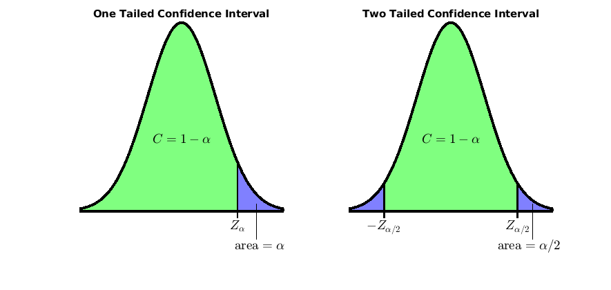
Fig. 4.17 One and two tailed 95% confidence intervals, \(\alpha = 0.05\), \(Z_\alpha = 1.645\), \(Z_{\alpha/2} = 1.96\).

Table 4.2 \(Z\)–critical values

	80%	85%	90%	95%	99%
\(Z_{\alpha/2}\)	1.28	1.44	1.645	1.96	2.576
\(Z_{\alpha}\)	0.84	1.04	1.282	1.645	2.326

We create 100 sampling sets in the simulation of a normal random variable listed in the testConfidence script. Using one of the samples, we find a 95% confidence interval. Our population mean is certainly within the confidence interval. Still, as you can see from the simulation output, the means of some samples are outside of our confidence interval.

% File: testConfidence.m
% Find a 95% confidence interval and see how many
% sample means are inside and outside the interval.
n = 100;
X = 50 + 20*randn(50, n);  % 50 x 100
X_bar = mean(X);
Za2 = 1.96;      % 95% Confidence
mu = mean(X(:))  % population mean
sigma = std(X(:));
% look at one sample
x_bar = X_bar(1);
Zlow = x_bar - Za2*sigma/sqrt(n)
Zhigh = x_bar + Za2*sigma/sqrt(n)
% test all samples
inAlpha = nnz(X_bar < Zlow | X_bar > Zhigh)
inC = nnz(X_bar > Zlow & X_bar < Zhigh)

>> testConfidence
mu =
    49.5914
Zlow =
    45.2956
Zhigh =
    53.5387
inAlpha =
    8
inC =
    92  % About as expected for a 95% confidence interval