3.4. 3-D Plots
MATLAB has several functions for plotting data in three dimensions.
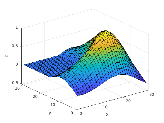
Try this code. The membrane data is built into MATLAB.
>> m = membrane;
>> surf(m)
>> xlabel('x')
>> ylabel('y')
>> zlabel('z')
|
|
Do you recognize the shape of the data?
Given only a matrix as input, the 3-D surface plotting functions will show the matrix values as the \(z\)–axis values and use the matrix indices for the \(x\)– and \(y\)–axis.
The meshgrid function is used to create matrices of the \(x\)– and
\(y\)–axis values that cover the range of data. Using data created from
meshgrid, the \(z\)–axis values are simple to create from
an equation.
>> x = -3:3;
>> y = -3:3;
>> [X, Y] = meshgrid(x,y);
>> X
X =
    -3    -2    -1     0     1     2     3
    -3    -2    -1     0     1     2     3
    -3    -2    -1     0     1     2     3
    -3    -2    -1     0     1     2     3
    -3    -2    -1     0     1     2     3
    -3    -2    -1     0     1     2     3
    -3    -2    -1     0     1     2     3
>> Y
Y =
    -3    -3    -3    -3    -3    -3    -3
    -2    -2    -2    -2    -2    -2    -2
    -1    -1    -1    -1    -1    -1    -1
     0     0     0     0     0     0     0
     1     1     1     1     1     1     1
     2     2     2     2     2     2     2
     3     3     3     3     3     3     3
>> Z = X.^2 + Y.^2
Z =
    18    13    10     9    10    13    18
    13     8     5     4     5     8    13
    10     5     2     1     2     5    10
     9     4     1     0     1     4     9
    10     5     2     1     2     5    10
    13     8     5     4     5     8    13
    18    13    10     9    10    13    18
3.4.1. 3-D Plot Functions
Here are descriptions of some of the 3-D plots available in MATLAB. Examples of
the plots are shown in Fig. 3.12 and Fig. 3.13. The data for
the plots is from the following code. Except for the plot3 function, the
X, Y, and Z data is a two dimension grid of values, such as
produced by the meshgrid function.
x = -8:0.25:8;
y = -8:0.25:8;
y1 = 8:-0.25:-8;
t = x.^2 + y1.^2;
z = (y1-x).*exp(-0.12*t); % for plot3
[X, Y] = meshgrid(x,y);
T = X.^2 + Y.^2;
Z = (Y-X).*exp(-0.12*T); % for surface plots

Fig. 3.12 Three dimensional plots: (a) surf, (b) surfc, (c) mesh, (d) plot3
- surf
surf(X, Y, Z): A three-dimensional surface plot. Probably the most often used 3-D plot function. Example shown in Fig. 3.12 (a). https://www.mathworks.com/help/matlab/ref/surf.html
- surfc
surfc(X, Y, Z): A contour plot under a surface plot. Example shown in Fig. 3.12 (b). https://www.mathworks.com/help/matlab/ref/surfc.html
- mesh
mesh(X, Y, Z): A wireframe mesh with color determined by Z, so color is proportional to surface height. Example shown in Fig. 3.12 (c). https://www.mathworks.com/help/matlab/ref/mesh.html
- plot3
plot3(x, y, z): A line plot, like theplotfunction, but in 3 dimensions. Example shown in Fig. 3.12 (d). https://www.mathworks.com/help/matlab/ref/plot3.html

Fig. 3.13 Three dimensional plots: (a) contour, (b) contour3, (c) meshz, (d) waterfall.
- contour
contour(X, Y, Z): A contour plot displays isolines to indicate lines of equal \(z\)–axis values, like found on a topographic map. Example shown in Fig. 3.13 (a). https://www.mathworks.com/help/matlab/ref/contour.html
- contour3
contour3(X, Y, Z): A 3-D contour plot. Not all data shows well with contour type plots. Example shown in Fig. 3.13 (b). https://www.mathworks.com/help/matlab/ref/contour3.html
- meshz
meshz(X, Y, Z): Like a mesh plot, with a curtain around the wireframe mesh. Example shown in Fig. 3.13 (c). https://www.mathworks.com/help/matlab/ref/meshz.html
- waterfall
waterfall(X, Y, Z): A mesh similar to the meshz function, but it does not generate lines from the columns of the matrices. Example shown in Fig. 3.13 (d). https://www.mathworks.com/help/matlab/ref/waterfall.html
- surfl
surfl(X, Y, Z): A shaded surface based on a combination of ambient, diffuse, and specular lighting models. Color is required for this plot to look right and the effect will vary depending on the data. An example plot is not shown. https://www.mathworks.com/help/matlab/ref/surfl.html
3.4.2. Axis Orientation
If the axes are not labeled, it may be hard to remember which is the \(x\)–axis and the \(y\)–axis. Use the right hand rule to help with this. Point your right index finger in the direction of the \(x\)–axis. Hold your middle finger at 90 degrees, which will be in the direction of the \(y\)–axis. Your thumb will be in the direction of the \(z\)–axis. See Fig. 3.14 for the correct 3-D coordinate frame layout.
A physical model is also helpful to visualize the 3-D coordinate frame axes. One can be printed on a 3-D printer. For a paper model, Peter Corke’s web-site has a PDF file that can be printed, cut, folded, and glued. The PDF file is available at http://www.petercorke.com/axes.pdf

Fig. 3.14 3-D coordinate frame and the right hand rule

Fig. 3.15 Right hand rule
