12.4.1. The Power Method
The power method is a technique to compute the most dominant eigenvalue of a
matrix. Although it is an old and simple algorithm, it is still used in
applications that require only one eigenpair. The basic theory of how the
algorithm works is based on a change of basis that occurs when a matrix is
raised to a specified power and multiplied by a vector,
 . Diagonalization of the matrix simplifies the
exponent calculation. It changes the basis of the coordinate system from an
Euclidean coordinate system to one that uses the matrix’s eigenvectors as the
basis vectors. This approach has several applications in addition to the power
method. See Change of Basis and Difference Equations for an explanation of using a change of basis
strategy in the analysis of difference equations.
. Diagonalization of the matrix simplifies the
exponent calculation. It changes the basis of the coordinate system from an
Euclidean coordinate system to one that uses the matrix’s eigenvectors as the
basis vectors. This approach has several applications in addition to the power
method. See Change of Basis and Difference Equations for an explanation of using a change of basis
strategy in the analysis of difference equations.
(12.5)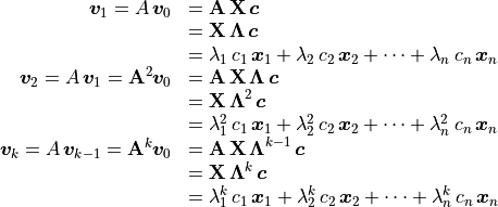
Solving for the linear coefficients is just a matter of solving a system
of linear equations:  , or in
MATLAB:
, or in
MATLAB: c = X\v. However, the power method does not calculate the
coefficients.
With the change of basis, the eigenvalues are the only variables raised
to the power  . The term with the largest eigenvalue,
 , will dominate the calculation. Terms associated with
eigenvalues having absolute values less than one go to zero when
becomes large. Since
, will dominate the calculation. Terms associated with
eigenvalues having absolute values less than one go to zero when
becomes large. Since 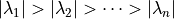 , the limit involves only one eigenvalue.
The vector  can be any vector of the same dimension as
the number of columns of
can be any vector of the same dimension as
the number of columns of  . If, for example,
 is a
is a  matrix, then
![\bm{v} = [1, 0]^T](../_images/math/99c8d5830280eeff9705c97bdb82feebcb737271.png) works. Find
works. Find  for a few values.
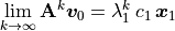
And if is large, the vectors are eigenvectors
scaled by
for a few values.
And if is large, the vectors are eigenvectors
scaled by  . You will know if is large enough or needs to be
increased after calculating several eigenvalues for different values of
. A simple equation determines the eigenvalue estimates.
Equation (12.6) makes a substitution of
. You will know if is large enough or needs to be
increased after calculating several eigenvalues for different values of
. A simple equation determines the eigenvalue estimates.
Equation (12.6) makes a substitution of
 to show that the calculation
finds the eigenvalue.
to show that the calculation
finds the eigenvalue.
(12.6)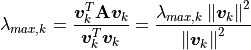
Note
Equation (12.6) is called the Rayleigh quotient after English physicist John William Rayleigh (1842–1919).
Here is an example of eigenvalue calculation.
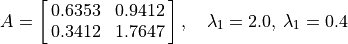
The first ten estimates of  are {1.4226, 1.905, 1.9839,
1.9969, 1.9994, 1.9999, 2, 2, 2, 2}. So, even without knowing the value
of the dominant eigenvalue, we observe that the iterative algorithm
converged at
are {1.4226, 1.905, 1.9839,
1.9969, 1.9994, 1.9999, 2, 2, 2, 2}. So, even without knowing the value
of the dominant eigenvalue, we observe that the iterative algorithm
converged at  . The rate at which the algorithm converges is
proportional to the ratio of the two largest eigenvalues
. The rate at which the algorithm converges is
proportional to the ratio of the two largest eigenvalues
 . In this small example, the
convergence was fast, but and
. In this small example, the
convergence was fast, but and  may
have similar magnitudes for large matrices, so quite a few more
iterations might be required before an accurate value is known.
may
have similar magnitudes for large matrices, so quite a few more
iterations might be required before an accurate value is known.
