14.7. The Flight of a Home Run Baseball
It was the bottom of the ninth inning of game 1 of the 2015 World Series. The New York Mets led the Kansas City Royals 4 to 3 with one out in the bottom of the ninth inning and then this happened. Watch the video and make note of two things – how long was the ball in the air (measure with a stop-watch), and estimate how far the ball went before hitting the ground. I used \(t_f = 5.9 seconds\). The marker on the wall gives us a starting point to estimate how far the ball went. I used \(x_f = 438 feet\).
You are to write a MATLAB script that will plot the vertical and horizontal path of the ball. Fig. 14.1 shows an example plot. The script should also display the maximum height, initial velocity, and initial projection angle of the ball. The steps listed below will guide you.
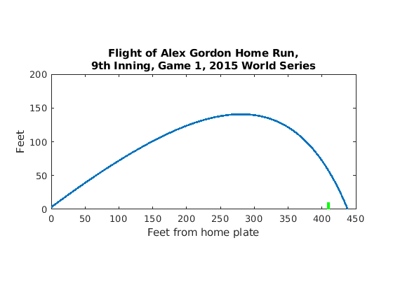
Fig. 14.1 Example Plot
The horizontal and vertical paths of the ball may be calculated independently.
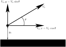
Fig. 14.2 The ball begins at an initial height. It has an initial velocity at an initial projection angle. The initial velocity may be split into horizontal and vertical components.
First make variables for constant values – gravity: \(g = -32 feet/sec^2\), final time of flight: \(t_f\) in seconds, Initial height: \(y_0 = 3 feet\), and the final horizontal displacement: \(x_f\) in feet. Also use
linspaceto make a 100 element vector, \(t\) for time from 0 to \(t_f\).The vertical path of the ball may be treated the same as for throwing a ball straight up. The only force on the ball worth noting is gravity. The height of the ball is given by
\[y = y_0 + V_{0,y}\,t + 1/2\,g\,t^2\]Using the \(t_f\) value measured with the stop watch, calculate \(V_{0,y}\), which occurs when \(y = 0\). The \(y\) path of the ball may be calculated now.
Next use the final horizontal displacement, \(x_f\), to calculate the initial horizontal velocity. Air resistance will slightly slow the horizontal displacement [ADAIR90] according to the differential equation,
\[\frac{dv_x(t)}{dt} = - 0.2\,v_x(t).\]The solution to the differential equation is
\[v_x(t) = V_{0,x}\,e^{-0.2\,t}.\]Then, the displacement comes from the definite integral of the velocity.
\[x(t) = V_{0,x}\int_0^t e^{-0.2 \tau} d\tau = 5\,V_{0,x}(1 - e^{-0.2\,t}).\]The constant value of 0.2 is an estimated, typical value. The real value is dependent on other factors such as the wind speed and direction that we don’t know.
From simple trigonometry, \(V_0\), and \(\theta\) can be expressed in terms of \(V_{0,y}\) and \(V_{0,x}\). Hint: Use the
atan2dfunction to find \(\theta\).Plot the path with a
'LineWidth'of 2.Show the home run wall by plotting a green line with
'LineWidth'of 3. Make the wall 10 feet tall at 410 feet from home plate.Remember to annotate the plot and to report the maximum height, initial velocity, and initial projection angle of the ball.
In addition, save the plot to a png file and submit it to the Canvas assignment page.
