2.11.1. Projections Onto a Line

A nice aspect of linear algebra is its geometric interpretation. That is, if we consider linear algebra problems in \(\mathbb{R}^2\) or \(\mathbb{R}^3\), then we can plot the vectors to depict the geometric relationships visually. Here, we consider vector projection, which gives us a geometric view of over-determined systems. We will begin with a simple example and later extend the concepts to higher dimensions.

Consider the following over-determined system where the unknown variable is a scalar.

\[\begin{split}\left\{\begin{matrix} 4x & = & 2 \\ 2x & = & 1 \end{matrix}\right.\end{split}\]

(2.25)\[\begin{split}\bm{a}\,x = \bm{b} \\\end{split}\]

\[\begin{split}\begin{bmatrix} 4 \\ 2 \end{bmatrix} \begin{bmatrix} x \end{bmatrix} = \begin{bmatrix} 2 \\ 1 \end{bmatrix}\end{split}\]

Figure Fig. 2.22 is a plot of the vectors \(\bm{a}\) and \(\bm{b}\).

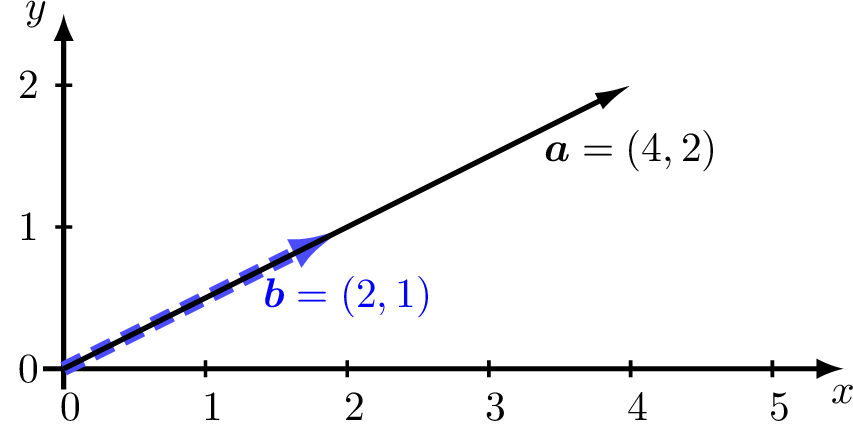
Fig. 2.22 Vectors \(\bm{a}\) and \(\bm{b}\) are consistent.

Here, \(x\) is a scalar, not a vector, and we can quickly see that \(x = 1/2\). But since \(\bm{a}\) and \(\bm{b}\) are vectors, we want to use a strategy that we can extend to matrices. We can multiply both sides of equation (2.25) by \(\bm{a}^T\) to turn the vectors into scalar dot products.

(2.26)\[\bm{a}^T \bm{a} x = \bm{a}^T \bm{b}\]

\[\begin{split}\begin{array}{rl} \begin{bmatrix} 4 & 2 \end{bmatrix} \begin{bmatrix} 4 \\ 2 \end{bmatrix} x &= \begin{bmatrix} 4 & 2 \end{bmatrix} \begin{bmatrix} 2 \\ 1 \end{bmatrix} \\ x &= \frac{10}{20} = \frac{1}{2} \end{array}\end{split}\]

Now, let’s extend the problem to a more general case as shown in figure Fig. 2.23 where vector \(\bm{b}\) is not necessarily inline with \(\bm{a}\). We will find a geometric reason to multiply both sides of equation (2.25) by \(\bm{a}^T\).

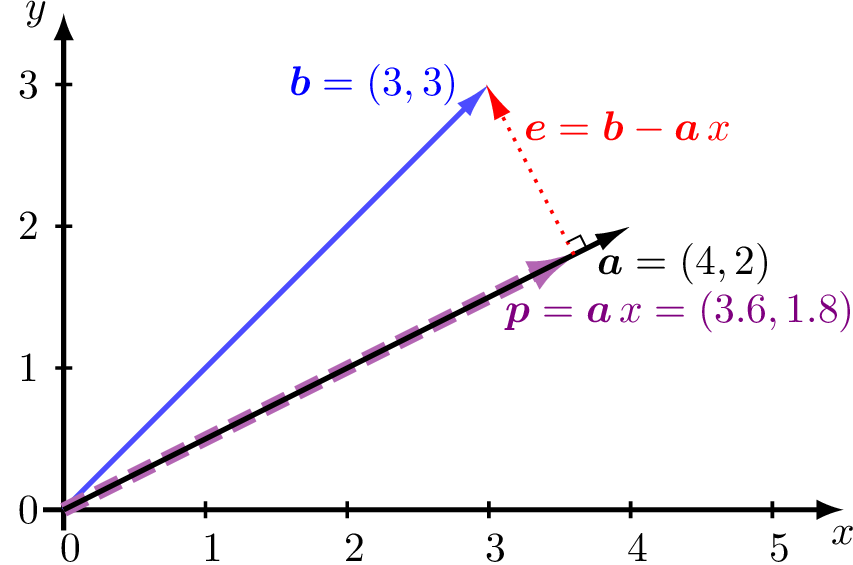
Fig. 2.23 Vector \(\bm{p}\) is a projection of vector \(\bm{b}\) onto vector \(\bm{a}\).

We wish to project the vector \(\bm{b}\) onto vector \(\bm{a}\), such that the error between \(\bm{b}\) and the projection is minimized. The projection, \(\bm{p}\), is a scalar multiple of \(\bm{a}\). That is, \(\bm{p} = \bm{a}\,x\), where \(x\) is the scalar value that we want to find. The error is the vector \(\bm{e} = \bm{b} - \bm{a}\,x\).

The geometry of the problem provides a simple solution for minimizing the error. The length of the error vector is minimized when it is perpendicular to \(\bm{a}\). Recall that two vectors are perpendicular (orthogonal) when their dot product equals zero.

\[\bm{a}^T\bm{e} = \bm{a}^T(\bm{b} - \bm{a}\,x) = 0\]

\[\bm{a}^T\bm{a}\,x = \bm{a}^T\bm{b}\]

(2.27)\[ \boxed{x = \frac{\bm{a}^T\bm{b}}{\bm{a}^T\bm{a}}}\]

Since \(x\) is a fraction of two dot products, we can think of the projection in terms of the angle, \(\theta\), between \(\bm{a}\) and \(\bm{b}\).

\[\begin{split}\begin{array}{rl} x &= \frac{\norm{\bm{a}}\,\norm{\bm{b}} \cos \theta}{\norm{\bm{a}}^2} \\ &\hfill \\ &= \frac{\norm{\bm{b}}}{\norm{\bm{a}}} \cos \theta \end{array}\end{split}\]

The projection is then:

\[\begin{split}\begin{array}{rl} \bm{p} &= \bm{a}\,x \\ &\hfill \\ &= \frac{\bm{a}}{\norm{\bm{a}}}\norm{\bm{b}} \cos\theta \\ &\hfill \\ &= \bm{a}\,\frac{\bm{a}^T\bm{b}}{\bm{a}^T\bm{a}} \end{array}\end{split}\]

We can also make a projection matrix, \(\bf{P}\), so that any vector may be projected onto \(\bm{a}\) by multiplying it by \(\bf{P}\).

\[\boxed{\mathbf{P} = \frac{\bm{a}\,\bm{a}^T}{\bm{a}^T\,\bm{a}}}\]

\[\bm{p} = \mathbf{P}\,\bm{b}\]

Note that \(\bm{a}\,\bm{a}^T\) is here a \(2{\times}2\) matrix and \(\bm{a}^T\,\bm{a}\) is a scalar. Here is an example.

In [16]: b = np.array([[3, 3]]).T; a = np.array([[4, 2]]).T

In [17]: P = (a @ a.T)/(a.T @ a) # Projection Matrix to a

In [18]: print(P)
[[0.8 0.4]
 [0.4 0.2]]

In [19]: p = P @ b; print(p)     # Projection of b onto a
[[3.6]
 [1.8]]

In [20]: x = (a.T @ b)/(a.T @ a); print(x) # length of projection
[[0.9]]

In [21]: e = b - p; print(e)     # error vector
[[-0.6]
 [ 1.2]]

In [22]: print(p.T @ e)          # Near zero dot product
[[-2.66453526e-15]]              # confirms e is perpendicular to p.