6.3.2. Homogeneous Matrix
Geometric translation is often added to the rotation matrix to make a homogeneous transformation matrix. The translation coordinates (\(x_t\) and \(y_t\)) are added in a third column. A third row is also added so that the resulting matrix is square.
The following matrix gives homogeneous rotation alone.
The following matrix gives a homogeneous translation alone.
The combined rotation and translation transformation matrix can be found by matrix multiplication.
6.3.3. Applying Transformations to a Point
When applied to a point, the homogeneous transformation matrix uses rotation followed by translation in the original coordinate frame. It is not translation followed by rotation.
>> R
R =
    0.5000   -0.8600         0
    0.8600    0.5000         0
    0         0         1.0000
>> Tt
Tt =
    1     0     1
    0     1     1
    0     0     1
>> % Define a point at (1.5, 1)
>> p = [1.5;1];
% Homogeneous coordinates
>> p1 = [p;1];
>> p2 = Tt*R*p1;
% Cartesian coordinates
>> p_new = p2(1:2)
p_new =
    0.8840
    2.7990
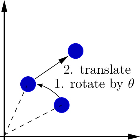
Fig. 6.14 A transformation applied to a point, \(\mathbf{p}_{2} = \mathbf{T}_t\,\mathbf{R}_{\theta}\,\mathbf{p}_1\), rotates and translates the point relative to the coordinate frame. The point in Cartesian coordinates is the first two values of the point in homogeneous coordinates.
In the following MATLAB session, we define a matrix and translation matrices using homogeneous coordinates. We compound the two with matrix multiplication and apply the compound transformation matrix to a point. Here, the rotation and translation matrices are constructed with a sequence of commands. Peter Corke’s Spatial Math Toolbox provides functions that expedite the effort [CORKE20]. [1]
>> % Rotation matrix
>> theta = pi/3;
>> R2=[cos(theta) -sin(theta);
       sin(theta) cos(theta)]
R2 =
    0.5000   -0.8660
    0.8660    0.5000
>> % homogeneous coordinates
>> R = [R2 [0; 0]; [0 0 1]]
R =
    0.5000  -0.8660        0
    0.8660   0.5000        0
         0        0   1.0000

>> % translation matrix
>> xt = 2; yt = 1;
>> tr = eye(3);
>> tr(1:2,3) = [xt; yt]
tr =
    1     0     2
    0     1     1
    0     0     1

>> % transformation matrix:
>> % pi/3 rotation,
>> % (2, 1) translation
>> T = tr*R
T =
    0.5000  -0.8660   2.0000
    0.8660   0.5000   1.0000
         0        0   1.0000

>> % point p at (1, 1)
>> % Cartesian coordinates
>> p = [1;1];
>> % Homogeneous coordinates
>> p1 = [p;1]
p1 =
    1
    1
    1

>> % transformation of p
>> p2 = T*p1
p2 =
    1.6340
    2.3660
    1.0000
>> % Cartesian coordinates
>> p_new = p2(1:2)
p_new =
    1.6340
    2.3660
Footnote:
