2.4.2. Homogeneous Matrix

Geometric translation is often added to the rotation matrix to make a homogeneous transformation matrix. The translation coordinates (\(x_t\) and \(y_t\)) are added in a third column. A third row is also added so that the resulting matrix is square.

\[\begin{split}\mathbf{T}(\theta, x_t, y_t) = \begin{bmatrix} \cos\theta & -\sin\theta & x_t \\ \sin\theta & \cos\theta & y_t \\ 0 & 0 & 1 \end{bmatrix}\end{split}\]

The following matrix gives homogeneous rotation alone.

\[\begin{split}\mathbf{R}(\theta) = \begin{bmatrix} \cos\theta & -\sin\theta & 0 \\ \sin\theta & \cos\theta & 0 \\ 0 & 0 & 1 \end{bmatrix}\end{split}\]

The following matrix gives a homogeneous translation alone.

\[\begin{split}\mathbf{T}_t(x_t, y_t) = \begin{bmatrix} 1 & 0 & x_t \\ 0 & 1 & y_t \\ 0 & 0 & 1 \end{bmatrix}\end{split}\]

The combined rotation and translation transformation matrix can be found by matrix multiplication.

\[\mathbf{T}(\theta, x_t, y_t) = \mathbf{T}_t(x_t, y_t) \, \mathbf{R}(\theta)\]

2.4.3. Applying Transformations to a Point

When applied to a point, the homogeneous transformation matrix uses rotation followed by translation in the original coordinate frame. It is not translation followed by rotation.

In [21]: import numpy as np

In [22]: theta = np.pi / 3

In [23]: R = np.array([[np.cos(theta),- np.sin(theta)],
    ...:               [np.sin(theta),np.cos(theta)]])

In [24]: R
Out[24]:
array([[ 0.5      , -0.8660254],
       [ 0.8660254,  0.5      ]])

In [25]: Tr = np.eye(3)

In [26]: Tr[:2, :2] = R

In [27]: Tr
Out[27]:
array([[ 0.5      , -0.8660254,  0.       ],
       [ 0.8660254,  0.5      ,  0.       ],
       [ 0.       ,  0.       ,  1.       ]])

In [28]: Tt = np.eye(3)

In [29]: Tt[:2, 2] = np.array([1, 1])

In [30]: Tt
Out[30]:
array([[1., 0., 1.],
       [0., 1., 1.],
       [0., 0., 1.]])

# Define a point at (1.5, 1)
In [31]: p = np.array([[1.5],[1]])

# Homogeneous coordinates
In [32]: p1 = np.vstack((p, [[1]]))

# Rotate
In [33]: Tr @ p1
Out[33]:
array([[-0.1160254 ],
       [ 1.79903811],
       [ 1.        ]])

# Translate
In [34]: p2 = Tt @ Out[33]
Out[34]:
array([[0.8839746 ],
       [2.79903811],
       [1.        ]])

# new point in Cartesian coordinates
In [35]: p_new = p2[[0, 1]]; p_new
Out[35]:
array([[0.8839746 ],
       [2.79903811]])

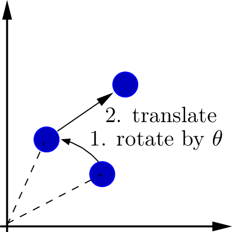
Fig. 2.14 A transformation applied to a point, \(\mathbf{p}_{2} = \mathbf{T}_t\,\mathbf{R}_{\theta}\,\mathbf{p}_1\), rotates and translates the point relative to the coordinate frame. The point in Cartesian coordinates is the first two values of the point in homogeneous coordinates.

Why do we say that rotation comes before translation?

The rotated and translated point is given by the product of two matrices and the original point location.

(2.9)\[\mathbf{p'} = \mathbf{T}_t(x_t, y_t) \, \mathbf{R}(\theta) \, \mathbf{p}\]

The left-to-right reading of equation (2.9) might lead one to say that the translation occurs before the rotation. We say that rotation occurs first because the rotation matrix is immediately left of the point location. So, the multiplication of the point by the rotation matrix moves the point first. Since multiplication of matrices is not commutative, the rotation matrix must be immediately left of the point location to get the desired result.

\[\mathbf{p'} = \underbrace{\mathbf{T}_t(x_t, y_t) \, \overbrace{\mathbf{R}(\theta)\, \mathbf{p}}^{\text{first product}}}_{\text{second product}}\]

In the following Python script, we define a matrix and translation matrices using homogeneous coordinates. We compound the two with matrix multiplication and apply the compound transformation matrix to a point. Here, the rotation and translation matrices are constructed with a sequence of commands. Peter Corke’s Spatial Math Toolbox provides functions that could expedite the effort [CORKE20]. [1]

# -*- coding: utf-8 -*-
"""
File: Homogeneous1.py
2D Rotation and translation of a point by homogeneous transformation matrix
"""

import numpy as np

# Rotation matrix
theta = np.pi / 3
R = np.array([[np.cos(theta),- np.sin(theta)],
            [np.sin(theta),np.cos(theta)]])
print(f'R = \n{R}\n')

# homogeneous coordinates
Tr = np.eye(3)  # Initialize as a 3x3 identity matrix
# Place the 2x2 rotation matrix in the top-left corner
Tr[:2, :2] = R
print(f'Tr (rotation only) = \n{Tr}\n')

# Translation only
xt = 2
yt = 1
tr = np.array([xt, yt])
print(f'tr = {tr}\n')
Tt = np.eye(3)
Tt[:2, 2] = tr
print(f'Tr (translation only) = \n{Tt}\n')

# transformation matrix:
# pi/3 rotation,
# (2, 1) translation
T = Tt @ Tr
print(f'T (transformation matrix) = \n{T}\n')

# Apply to a point, p = (1, 1)
p = np.array([[1],[1]])
# Homogeneous coordinates
p1 = np.vstack((p, [[1]]))
p2 = T @ p1
print(f'p2 = \n{p2}\n')
p_new = p2[np.arange(0,2)]
print(f'p_new rotated from (1, 1) = \n{p_new}\n')

Output from the script follows.

R =
[[ 0.5       -0.8660254]
 [ 0.8660254  0.5      ]]

Tr (rotation only) =
[[ 0.5       -0.8660254  0.       ]
 [ 0.8660254  0.5        0.       ]
 [ 0.         0.         1.       ]]

tr = [2 1]

Tr (translation only) =
[[1. 0. 2.]
 [0. 1. 1.]
 [0. 0. 1.]]

T (transformation matrix) =
[[ 0.5       -0.8660254  2.       ]
 [ 0.8660254  0.5        1.       ]
 [ 0.         0.         1.       ]]

p2 =
[[1.6339746]
 [2.3660254]
 [1.       ]]

p_new rotated from (1, 1) =
[[1.6339746]
 [2.3660254]]

2.4.4. Transform Functions

For our future use, we define functions to provide rotation and translation transformation matrices.

# -*- coding: utf-8 -*-
"""
File: transforms2d.py

2D spatial transforms:
    rot2d - 2x2 rotation matrix
    hrot2d - 3x3 rotation homogeneous transform
    transl2d - 3x3 translation homogeneous transform

"""
import numpy as np

def rot2d(theta: float, deg: bool = False) -> np.array:
    if deg:
        theta = theta * (np.pi / 180)
    c = np.cos(theta)
    s = np.sin(theta)
    R = np.array([[c, -s], [s, c]])
    return R

def hrot2d(theta: float, deg: bool = False) -> np.array:
    if deg:
        theta = theta * (np.pi / 180)
    c = np.cos(theta)
    s = np.sin(theta)
    R = np.array([[c, -s, 0], [s, c, 0], [0, 0, 1]])
    return R

def transl2d(x: float, y: float) -> np.array:
    T = np.eye(3)
    T[0][2] = x
    T[1][2] = y
    return T

if __name__ == '__main__':
    print(f'Rot pi/3:\n{rot2d(np.pi/3)}')
    print(f'Rot 30 deg:\n{rot2d(30, True)}')
    print(f'Homogeneous Rot pi/3:\n{hrot2d(np.pi/3)}')
    print(f'Homogeneous Rot 30 deg:\n{hrot2d(30, True)}')
    print(f'translate (2, 1):\n{transl2d(2, 1)}')

Footnote:

[1]

You might also be interested in his toolboxes for robotics and machine vision.